In the last post we built a neural network by stacking layers. But there was a catch - stacking linear layers without anything between them is mathematically the same as having one layer. This post explains why that’s a problem and how activation functions fix it.
Why it exists
A linear layer computes: output = input × W + b. Stack two of them and the whole thing still simplifies to input × W + b - just with different numbers. The math collapses. No matter how many linear layers you stack, it’s equivalent to one. The code in the walkthrough section proves this directly if you want to see it.
The depth buys you nothing.
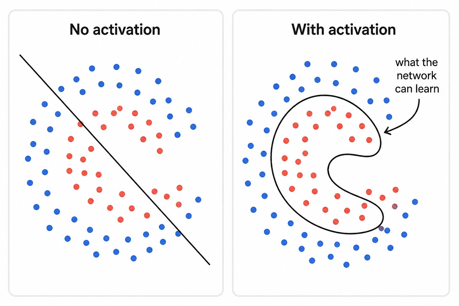
This is a real problem. Most things you want to learn aren’t linear. The relationship between a sentence and its sentiment isn’t a straight line. Neither is the relationship between pixels and whether an image contains a cat.
The fix is to put a non-linear function between each layer. That function is called an activation function.
How it works
An activation function takes a single number and transforms it. After each layer’s matrix multiplication, you run every output through the activation function before passing it to the next layer. That one step breaks the linearity - two linear layers with an activation between them can no longer be collapsed into one.
The story of activation functions is a chain of problem and fix. Each one was invented to solve a problem with the previous one.
Sigmoid and tanh - the originals
Sigmoid: f(x) = 1 / (1 + e^(-x)) - squashes any input to a value between 0 and 1. Tanh: f(x) = (e^x - e^(-x)) / (e^x + e^(-x)) - squashes to between -1 and 1. Both are smooth curves and worked fine as the first non-linearities.
Pro: Smooth, differentiable everywhere, output is bounded and interpretable (sigmoid outputs a probability-like value).
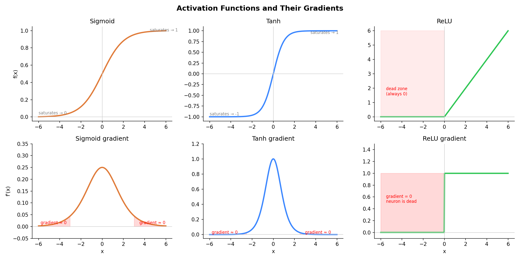
Con: Vanishing gradients. When inputs are large or small, the curve flattens out - the gradient becomes nearly zero. During training, gradients flow backwards through each layer. When they pass through a saturated sigmoid, they get multiplied by a near-zero number and shrink. Do this across many layers and the gradient reaches the early layers as almost nothing. Those layers stop learning.
You’ll still see sigmoid in specific spots - binary classification output layers and inside LSTM gates (post 1.8). But not as a general activation in deep networks.
The plot below shows all three activations and their gradients. The red shaded regions are where the gradient collapses to near zero - for sigmoid and tanh this happens at both ends (saturated region), and for ReLU it’s the entire negative half (dead zone).
ReLU - fixed vanishing gradients
ReLU (Rectified Linear Unit): f(x) = max(0, x).
Negative values become zero. Positive values pass through unchanged. It’s Math.max(0, x) applied to every number in the output.
Pro: For positive values the gradient is always 1 - it never shrinks. This fixed the vanishing gradient problem and made training deep networks practical. It’s also very fast to compute.
Con: Dying ReLU. If a neuron’s inputs are always negative, ReLU always outputs zero. A gradient of zero means the weights never update. The neuron is dead - stuck at zero forever. In large networks, a significant portion of neurons can die this way, especially with high learning rates.
GELU - fixed dying ReLU
GELU (Gaussian Error Linear Unit): f(x) = x × Φ(x) where Φ(x) is the cumulative distribution function of the standard normal distribution. In practice this is approximated as 0.5 × x × (1 + tanh(√(2/π) × (x + 0.044715 × x³))). The formula looks intimidating but the intuition is simple - instead of a hard cutoff at zero, it tapers off gradually. Small negative values get dampened rather than zeroed out completely, so neurons are less likely to die.
Pro: Smooth curve means no hard zero, so neurons don’t die. Performs better than ReLU on language tasks in practice. Used in BERT, GPT-2, and GPT-3.
Con: Slightly more expensive to compute than ReLU. And as model architectures evolved further, SiLU was found to work just as well or better.
SiLU - a smoother alternative
SiLU (Sigmoid Linear Unit), also called Swish: f(x) = x × sigmoid(x) where sigmoid(x) = 1 / (1 + e^(-x)). Like GELU, it’s smooth and lets small negative values partially pass through.
Pro: Similar benefits to GELU - no dying neurons, smooth gradients. Found to outperform both ReLU and GELU on larger models. Used in LLaMA, Mistral, Gemma, and most open-source LLMs today.
Con: Marginally more compute than ReLU, though the difference is negligible in practice.
A quick summary of the evolution:
| Activation | Solves | Problem it introduced |
|---|---|---|
| Sigmoid / tanh | Non-linearity | Vanishing gradients in deep networks |
| ReLU | Vanishing gradients | Dying neurons |
| GELU / SiLU | Dying neurons | Slightly more compute (minor) |
Code
Step 1 - show that two linear layers with no activation collapse into one:
import torch
import torch.nn as nn

# Two separate layers
layer1 = nn.Linear(4, 4, bias=False)
layer2 = nn.Linear(4, 4, bias=False)

# One combined layer with the same weight product
combined = nn.Linear(4, 4, bias=False)
combined.weight.data = layer2.weight.data @ layer1.weight.data

x = torch.randn(1, 4)

out_two   = layer2(layer1(x))
out_one   = combined(x)

print("Two layers: ", out_two.detach().round(decimals=4))
print("One layer:  ", out_one.detach().round(decimals=4))
print("Same?", torch.allclose(out_two, out_one, atol=1e-5))
Two layers: tensor([[ 0.3412, -0.1209, 0.8801, -0.2341]])
One layer: tensor([[ 0.3412, -0.1209, 0.8801, -0.2341]])
Same? TrueTwo layers, same output as one. The depth added nothing.
Step 2 - add ReLU between the same layers and the outputs diverge:
out_with_relu = layer2(torch.relu(layer1(x)))
out_one       = combined(x)

print("With ReLU:    ", out_with_relu.detach().round(decimals=4))
print("Without ReLU: ", out_one.detach().round(decimals=4))
print("Same?", torch.allclose(out_with_relu, out_one, atol=1e-5))
With ReLU: tensor([[ 0.5123, -0.0447, 0.9012, -0.1803]])
Without ReLU: tensor([[ 0.3412, -0.1209, 0.8801, -0.2341]])
Same? FalseSame input, same weights - one ReLU call between the layers and they no longer produce the same result.
Step 3 - plot ReLU, GELU, SiLU side by side:
import matplotlib.pyplot as plt
import torch
import torch.nn.functional as F

x = torch.linspace(-4, 4, 200)

plt.figure(figsize=(10, 3))
plt.plot(x, F.relu(x),  label="ReLU",  linewidth=2)
plt.plot(x, F.gelu(x),  label="GELU",  linewidth=2)
plt.plot(x, F.silu(x),  label="SiLU",  linewidth=2)
plt.axhline(0, color="gray", linewidth=0.5)
plt.axvline(0, color="gray", linewidth=0.5)
plt.legend()
plt.title("Activation Functions")
plt.tight_layout()
plt.savefig("activation-functions.png", dpi=150)
plt.show()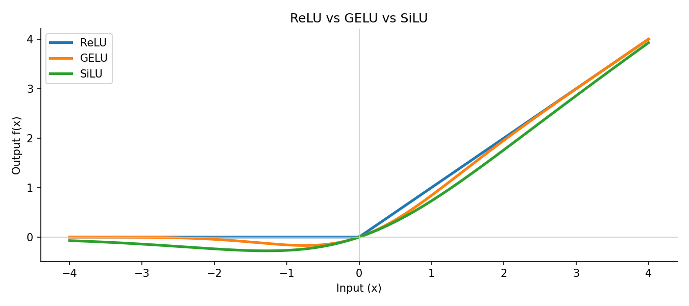
Notice how ReLU has a hard corner at zero while GELU and SiLU curve smoothly. SiLU dips slightly negative before zero - that small allowance for negative values is part of why it works well in practice.
Key takeaways
- Stacking linear layers without anything between them is equivalent to one linear layer - depth alone adds nothing
- Activation functions break the linearity, letting the network learn curved and complex patterns
- ReLU is the default for most things; GELU is standard in transformer-based models; SiLU is used in most modern open-source LLMs like LLaMA
What to read next
Now that the network can compute non-linear functions, we need a way to measure how wrong its predictions are. That measurement is the loss function - the signal that tells the network what to fix.