What is a Neural Network?

Why neural networks exist

Programs used to be explicit rules. To detect spam email you’d write: if the message contains “free money”, flag it. If it mentions “Nigerian prince”, flag it. Add more rules as spammers adapt.

This breaks down fast. Language is too varied. You end up with thousands of rules that still miss half the spam.

Machine learning flips the approach. Instead of writing rules, you show the program thousands of examples - spam emails and legitimate ones - and let it figure out the patterns itself.

A neural network is the most common tool for this. It’s a function that takes inputs and produces an output. What makes it powerful is that its internal parameters - called weights - are learned from data, not written by hand.

This setup - learning from labelled examples - is called supervised learning. It’s one of three training approaches; the others (unsupervised and self-supervised) come up later when we get to how LLMs are pre-trained.

The intuition

Start with the smallest piece: a single neuron.

A neuron takes a list of numbers, multiplies each by a weight, sums them up, and outputs one number. That’s it.

Think of it like a panel of judges scoring a dish. Each judge has an opinion (a number) and a level of influence (a weight). The final score is the weighted sum of all their opinions. A judge with a high weight swings the result more than one with a low weight.

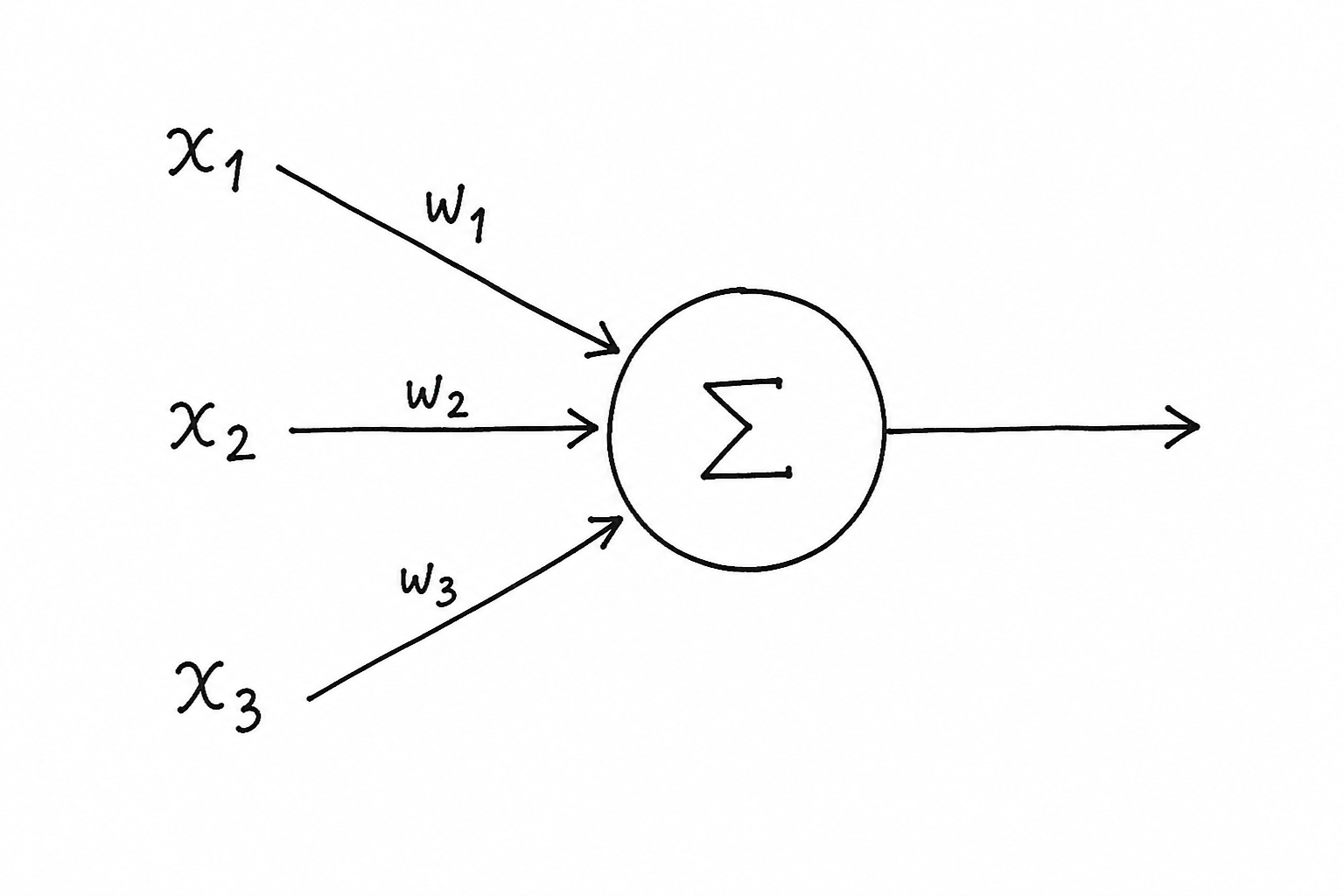
The formula written out:

output = (x₁ × w₁) + (x₂ × w₂) + (x₃ × w₃) + b

b is the bias - a constant added to shift the result. Think of it like the +c intercept in a line equation y = mx + c. It lets the neuron fire even when all inputs are zero.

How it works

A single neuron can only draw one straight line through data. It cannot learn anything curved or complex on its own. The solution is to combine many neurons and stack them in layers.

A layer is a group of neurons that all receive the same input. Each neuron in the layer produces its own output, so a layer with 4 neurons turns one input vector into 4 numbers. Under the hood this is a matrix multiplication - the input vector gets multiplied by a weights matrix. If the input has 3 values and the layer has 4 neurons, the weights matrix is shape (3×4) and the output is a 4-element vector.

A neural network stacks layers one after another. The output of one layer becomes the input of the next. It’s function composition: layer3(layer2(layer1(x))).

The first layer is called the input layer - it receives your raw data. The last is the output layer - it produces the prediction. Everything in between is a hidden layer. “Hidden” just means you don’t directly see its outputs; they’re internal computations.

Each layer picks up on something different. In an image network, the first layer might detect edges, the second combines edges into shapes, the third recognises objects. You don’t write any of this - the weights figure it out from data.

The forward pass is the process of pushing one input through all layers from left to right to get a prediction. Data goes in, flows through each layer in order, and comes out the other end as a result.

Right now the weights are random, so the output is garbage. How to fix that - adjusting weights so the network gets things right - is covered in post 1.4. For now, focus on the shape: data in, each layer transforms it, prediction out.

One thing to keep in mind: stacking more linear layers doesn’t actually make the network more powerful on its own. Two linear transformations back to back are still just one linear transformation. That’s why real networks put something between each layer to break the pattern. The next post covers what that something is.

Code

Step 1 - a single neuron in plain Python, no libraries:

inputs  = [1.0, 2.0, 3.0]
weights = [0.5, -0.3, 0.8]
bias    = 0.1

output = sum(x * w for x, w in zip(inputs, weights)) + bias
print(output)

3.4

0.5×1.0 + (−0.3)×2.0 + 0.8×3.0 + 0.1 = 0.5 − 0.6 + 2.4 + 0.1 = 2.4. The math is nothing more than multiply and sum.

Step 2 - the same operation using PyTorch’s nn.Linear:

import torch
import torch.nn as nn

layer  = nn.Linear(in_features=3, out_features=1)
x      = torch.tensor([[1.0, 2.0, 3.0]])
output = layer(x)

print(output.shape)
print(output)

torch.Size([1, 1])
tensor([[0.47]], grad_fn=<AddmmBackward0>)

The output value differs from step 1 because nn.Linear initialises weights randomly. The shape [1, 1] means one sample, one output value. grad_fn on the tensor means PyTorch is already tracking this operation for backpropagation - more on that in post 1.4.

Step 3 - a 3-layer network, forward pass, watch the shape change at each layer:

model = nn.Sequential(
    nn.Linear(3, 4),  # 3 inputs → 4 outputs
    nn.Linear(4, 2),  # 4 inputs → 2 outputs
    nn.Linear(2, 1),  # 2 inputs → 1 output
)

x = torch.tensor([[1.0, 2.0, 3.0]])

for i, layer in enumerate(model):
    x = layer(x)
    print(f"After layer {i + 1}: shape = {x.shape}")

After layer 1: shape = torch.Size([1, 4])
After layer 2: shape = torch.Size([1, 2])
After layer 3: shape = torch.Size([1, 1])

Three inputs squeeze down to one prediction through three transformation steps. The weights controlling those transformations are currently random. Training is the process of adjusting them until the final output matches the correct answer.

Key takeaways

• A neuron multiplies each input by a weight, sums the results, and adds a bias - one number in per input, one number out
• A neural network is layers of neurons stacked in sequence, each layer’s output feeding the next
• The forward pass runs data left-to-right through every layer to produce a prediction; at this point weights are random - learning how to update them comes in post 1.4

What to read next

Stacking linear layers alone doesn’t give you a more powerful network. You need something between each layer to make the stacking useful - that something is called an activation function.

The next post explains why, and covers the three you’ll see in almost every modern model: ReLU, GELU, and SiLU.

→ Post 1.2 - Activation Functions: Why ReLU, GELU, and SiLU Exist