In post 1.7 we saw that a model can memorise training data and fail on anything new. Dropout was the fix. But there’s a deeper question underneath: why do models fail in the first place? It turns out there are exactly two ways a model can be wrong, and they pull in opposite directions. Understanding them tells you what to do when training isn’t working.
Why it exists
Every model makes errors on data it hasn’t seen. Some of that error is unavoidable — the world is noisy. But the rest comes from one of two failure modes.
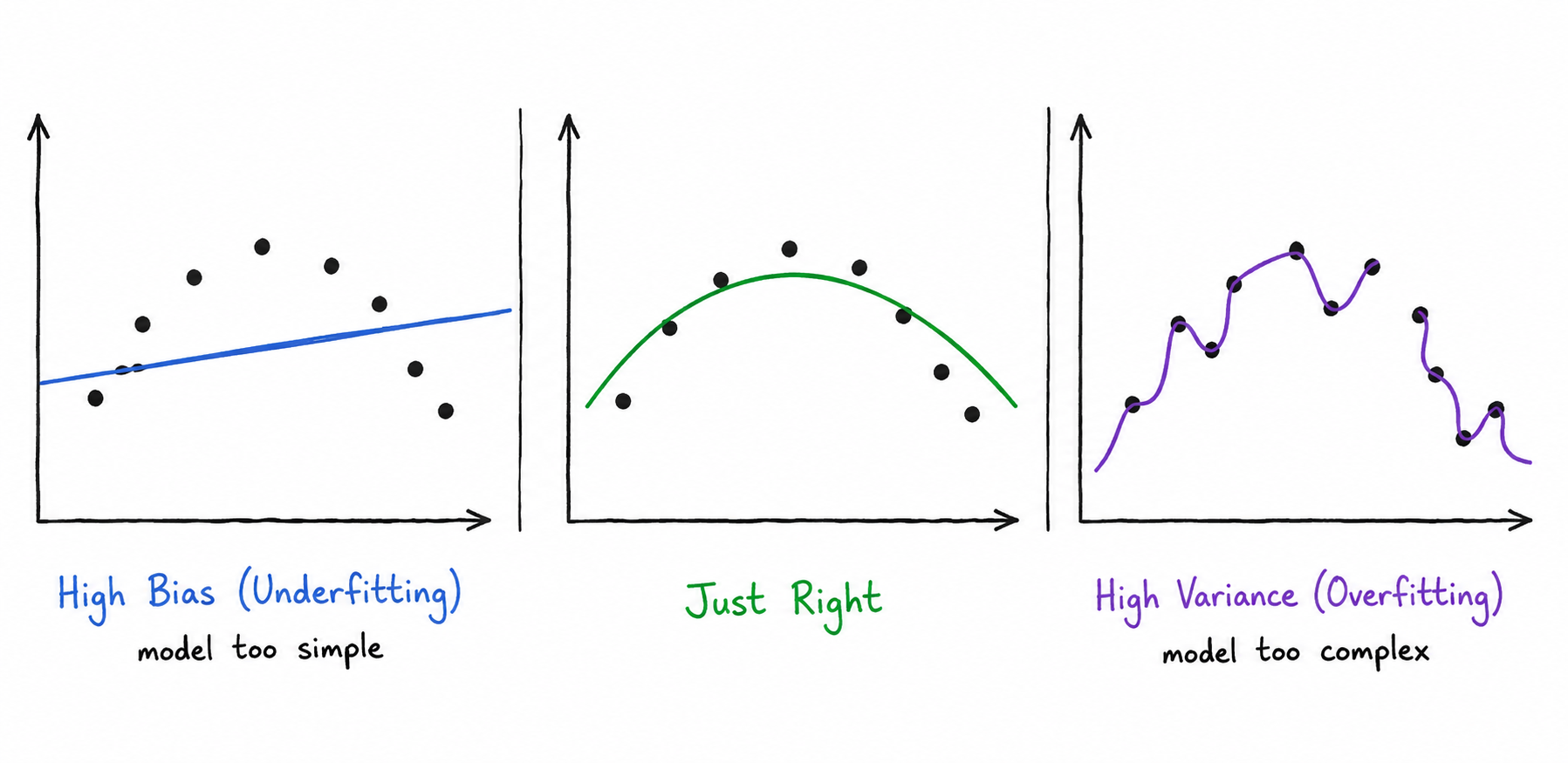
The first is being too simple. A model that assumes a straight-line relationship between input and output will be wrong even if you gave it infinite training data, because reality isn’t a straight line. It doesn’t matter which samples you train on — the model is fundamentally wrong. This is bias. High bias means the model has wrong assumptions baked in. It underfits — it misses the true pattern entirely.
The second is being too sensitive. A model that memorises every training sample perfectly will perform well on those exact samples and poorly on everything else. Change which samples you train on and you get a completely different model. This is variance. High variance means the model is too sensitive to the specific data it was trained on. It overfits — it learns the noise, not the signal.
These aren’t just abstract categories. They tell you what to fix when something goes wrong:
| Symptom | Likely cause | Fix |
|---|---|---|
| High training error AND high validation error | High bias (underfitting) | Use a bigger model |
| Low training error, high validation error | High variance (overfitting) | Regularise, get more data |
How it works
Bias
Bias is the error that comes from the model’s assumptions being wrong.
A linear model (y = wx + b) can only fit straight lines. Give it data that follows a curve and it will always miss — not because it hasn’t trained enough, but because its architecture won’t let it represent the right answer. This is a high-bias model. More data doesn’t help. More training steps don’t help. The model needs to be more expressive.
Think of integer division in code. 7 / 2 gives 3, always. No matter how many examples you show it, it will never give you 3.5. The bias is built into the operation itself.
Variance
Variance is the error that comes from the model being too sensitive to the specific training samples.
A very large network trained on a small dataset will find a set of weights that fits every training point exactly — including the noise in those measurements. Those noisy details don’t generalise to new data. If you retrained the same model on a slightly different set of 60 samples, you’d get completely different predictions. The model’s output is unstable — it varies with the data.
This is a lookup table problem. A lookup table that maps every training input to its exact output will hit 100% on training. But ask it about an input it’s never seen and it has nothing to return. All it learned was the exact keys it was given.
The tradeoff
As you make a model more complex — more layers, more neurons — bias falls. The model can represent more shapes, fit more patterns. But variance rises. A model with more capacity can memorise more, and memorisation increases sensitivity to training data.
The plot below shows this directly. Train a two-layer network on 25 points from a sine curve. Vary only the width of the hidden layers — from a single linear layer up to 256 neurons:
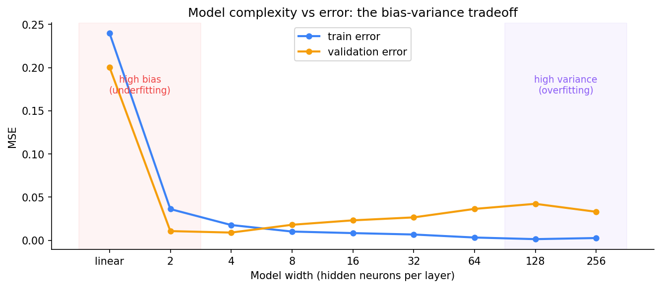
The linear model (far left) has both train and validation error high — it can’t fit the sine curve at all. Too simple. As we add neurons, both errors drop and the model starts capturing the real pattern. Validation error bottoms out around width 4. Past that, train error keeps falling — the model memorises more — while validation error climbs, because what it’s memorising is noise.
The sweet spot is in the middle: complex enough to capture the signal, simple enough not to memorise the noise.
Where this matters in practice
Diagnosing training problems:
When a model isn’t working, the first thing to check is where the error is. If training error is high, you have a bias problem — the model can’t fit the data. Add capacity: more layers, more neurons, a different architecture. If training error is low but validation error is high, you have a variance problem — add regularisation (dropout, weight decay), get more data, or simplify the model.
Modern deep learning changed the picture:
The classical tradeoff suggests you have to pick a point on the bias-variance curve. But large neural networks with good regularisation can break this intuition — they have low bias (they’re expressive enough to fit anything) AND controlled variance (regularisation prevents them from memorising too specifically).
GPT-4, LLaMA, and similar models have billions of parameters — high capacity, should overfit. But they’re trained on so much data, with enough regularisation, that the variance is managed. The tradeoff still exists. It’s just managed with better tools than simply choosing a small model.
The practical rule of thumb: start with a model large enough to fit the training data (get bias low), then add regularisation to pull variance back in. Don’t start with a tiny model hoping to avoid overfitting — an underfit model is just as broken as an overfit one, and harder to diagnose.
Code
Step 1 - reproduce the complexity curve:
import torch
import torch.nn as nn
import numpy as np
import matplotlib.pyplot as plt

torch.manual_seed(42)

N = 25
X_train = torch.linspace(0, 1, N).unsqueeze(1)
y_train = torch.sin(2 * np.pi * X_train) + 0.15 * torch.randn_like(X_train)
X_val   = torch.linspace(0, 1, 300).unsqueeze(1)
y_val   = torch.sin(2 * np.pi * X_val)   # clean sine — no noise

def make_model(width):
    if width == 0:
        return nn.Linear(1, 1)  # purely linear — maximum bias
    return nn.Sequential(
        nn.Linear(1, width), nn.Tanh(),
        nn.Linear(width, width), nn.Tanh(),
        nn.Linear(width, 1),
    )

widths = [0, 2, 4, 8, 16, 32, 64, 128, 256]
loss_fn = nn.MSELoss()
train_errors, val_errors = [], []

for w in widths:
    torch.manual_seed(0)
    model = make_model(w)
    opt   = torch.optim.Adam(model.parameters(), lr=3e-3)

    for _ in range(3000):
        model.train()
        loss = loss_fn(model(X_train), y_train)
        opt.zero_grad(); loss.backward(); opt.step()

    model.eval()
    with torch.no_grad():
        train_errors.append(loss_fn(model(X_train), y_train).item())
        val_errors.append(loss_fn(model(X_val), y_val).item())

for w, tr, vl in zip(widths, train_errors, val_errors):
    print(f"width={str(w):>4}  train={tr:.4f}  val={vl:.4f}")
width= 0 train=0.2400 val=0.2005
width= 2 train=0.0362 val=0.0107
width= 4 train=0.0177 val=0.0090
width= 8 train=0.0102 val=0.0180
width= 16 train=0.0084 val=0.0231
width= 32 train=0.0067 val=0.0266
width= 64 train=0.0032 val=0.0364
width= 128 train=0.0014 val=0.0423
width= 256 train=0.0027 val=0.0330Train error falls monotonically as width grows. Validation error reaches its minimum at width 4, then rises — the model is memorising the noise in the 25 training points. Width 4 is the sweet spot for this particular problem.
Step 2 - diagnose a model using train vs val error:
# high bias: both errors are high
print(f"Linear model  — train: {train_errors[0]:.4f}  val: {val_errors[0]:.4f}")

# good fit: both errors are low and close
print(f"Width 4       — train: {train_errors[2]:.4f}  val: {val_errors[2]:.4f}")

# high variance: train low, val high
print(f"Width 256     — train: {train_errors[-1]:.4f}  val: {val_errors[-1]:.4f}")
Linear model — train: 0.2400 val: 0.2005
Width 4 — train: 0.0177 val: 0.0090
Width 256 — train: 0.0027 val: 0.0330The diagnostic pattern:
- Both errors high → increase model capacity
- Train low, val high → add regularisation or more data
- Both errors low and close → you’re in the right zone
Key takeaways
- Bias is error from wrong assumptions — the model is too simple to capture the true pattern. Fix by adding capacity.
- Variance is error from sensitivity to training data — the model memorises instead of generalising. Fix with regularisation or more data.
- The practical workflow: make the model large enough to fit training data first (control bias), then regularise to bring validation error down (control variance).
What to read next
We’ve covered all the core building blocks of deep learning. The next two posts step back to look at the architectures that came before Transformers — and why each one hit a wall that eventually made a new approach necessary.
→ Post 1.9 - CNN, RNN, LSTM: The Road to Transformers