In post 1.6 we added normalisation to keep activations stable across layers. Training is now stable. But there’s a different failure mode that shows up once training works well: the model starts memorising the training data instead of learning from it. This post is about that problem and the main technique used to fix it.
Why it exists
Imagine you’re studying for an exam by memorising every past paper question word for word. On those exact questions, you’d score 100%. On any new question — same topic, different wording — you’d struggle because you never learned the underlying concepts, just the specific phrasing.
Neural networks do the same thing. Given enough capacity and enough training, a model will memorise the training examples rather than learn the pattern behind them. It performs perfectly on training data and badly on anything it hasn’t seen before. This is overfitting.
The visible signal is a gap between training and validation accuracy. Validation data is held out during training — the model never sees it. If training accuracy is 100% and validation accuracy is 70%, the model is memorising, not generalising.
Think of it as cache keys that are too specific. A cache lookup that matches on the exact input string will hit perfectly for known inputs and miss on every slight variation. What you want is a cache that matches on the underlying intent — a broader key that hits for inputs with the same meaning.
Regularisation is the umbrella term for techniques that discourage memorisation and push the model toward learning broader patterns. Dropout is the most common one in deep learning.
How it works
Overfitting in practice
A small dataset makes overfitting easy to trigger. Train a two-layer network on 60 samples with 20 features, where only 2 features actually determine the label. The network has 256 neurons per layer — far more capacity than the problem needs.
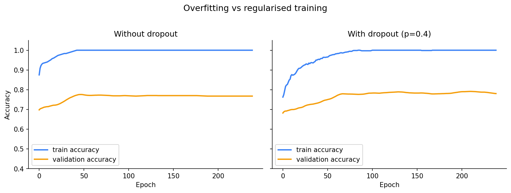
The model quickly reaches 100% training accuracy — it has memorised all 60 samples. But validation accuracy plateaus around 77%. The 23-point gap is overfitting.
Dropout
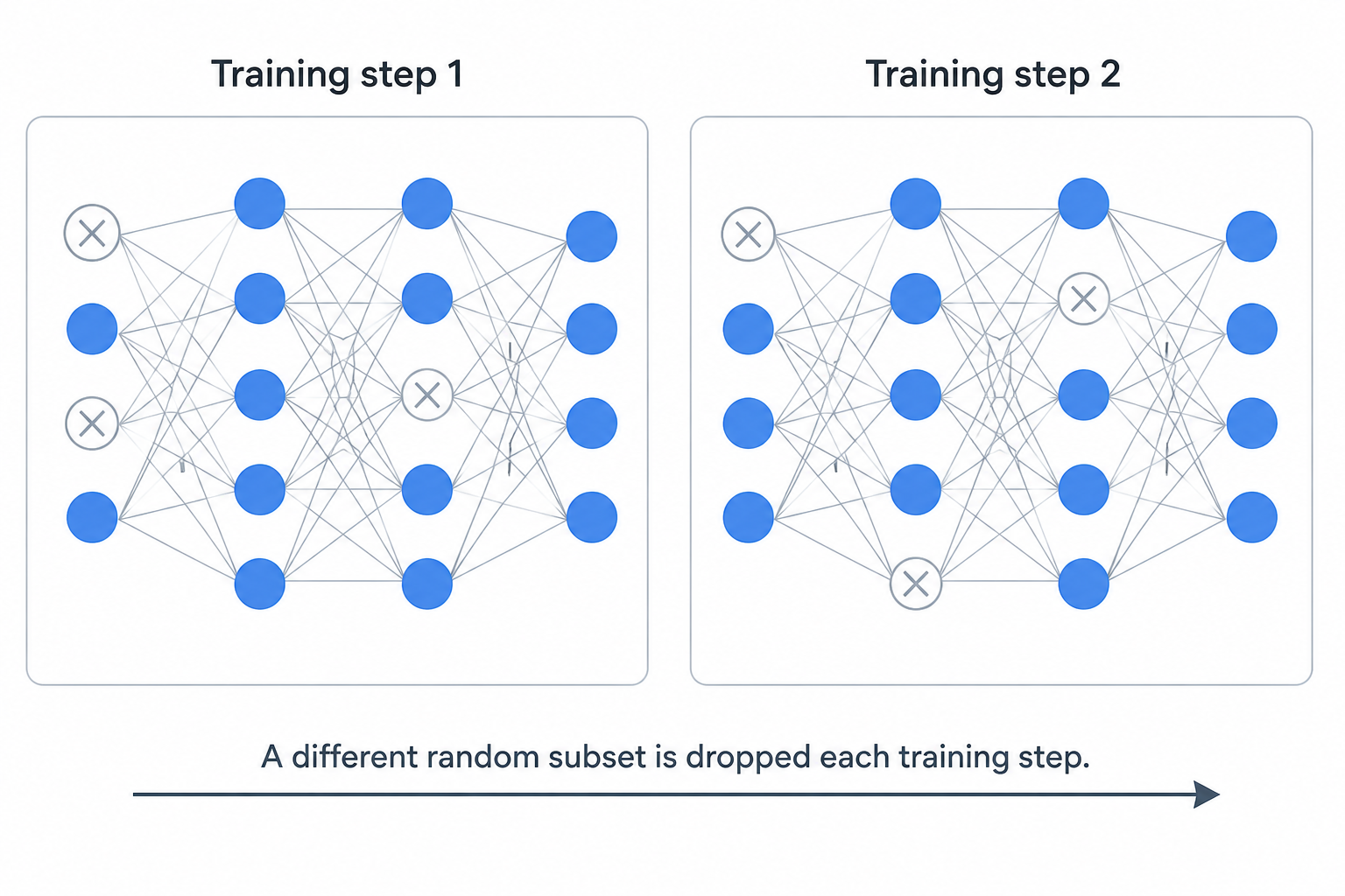
Dropout is simple in principle. During each training step, randomly zero out a fraction of neurons. If you set p=0.4, each neuron has a 40% chance of being zeroed out for that step — its output is set to zero, and the gradient doesn’t flow through it.
The fraction of neurons dropped is the dropout rate, written as p. Common values are 0.1 to 0.5.
Why does this help? A network without dropout can develop co-adaptation: neuron A learns to output the right value, and neuron B learns to amplify A’s output. They work together as a pair. If you always remove a random half of neurons during training, no single neuron or pair can be relied on to always be present. The network is forced to build redundancy instead — each neuron needs to carry useful information on its own, because it can’t count on its neighbours.
This is the same thinking behind chaos engineering in distributed systems. You randomly kill nodes during testing so the system can’t develop hidden dependencies on any single node. Netflix’s Chaos Monkey does exactly this: kill a random server, see if the system survives. Dropout is chaos engineering for your neurons.
The right panel in the plot shows the effect: training accuracy rises more slowly (the network can’t memorise as fast) and the train-val gap shrinks. The model generalises better.
Dropout at inference
Dropout is only active during training. At inference time, all neurons are on.
But there’s a catch: during training, an average of p fraction of neurons are zeroed out at each step. If you suddenly turn them all on at inference, the activations will be scaled differently — you’d be adding back neurons that were never present during training, inflating the output magnitudes.
PyTorch handles this automatically with inverted dropout: during training, the outputs of surviving neurons are scaled up by 1/(1-p) to compensate for the ones that were dropped. At inference, no scaling is needed since all neurons are active and the magnitudes match.
You never need to change anything in your code between training and inference — calling model.eval() and model.train() is enough.
Weight decay revisited
Dropout isn’t the only regulariser. Weight decay — covered briefly in post 1.5 as part of AdamW — is the other common one. It adds a penalty to the loss for large weights, nudging the model toward solutions with smaller weight values. Smaller weights produce smoother functions that generalise better.
In practice: use AdamW (which includes weight decay) for transformers and LLMs, and add dropout in the attention and feed-forward layers at a low rate (0.1). For smaller models on small datasets, higher dropout (0.2–0.5) helps more.
Modern very large models (70B+ parameters) often use little or no dropout — at that scale, the amount of data relative to the model is large enough that memorisation is less of a concern.
Code
Step 1 - reproduce overfitting:
import torch
import torch.nn as nn

torch.manual_seed(42)

# tiny dataset: 60 samples, 20 features, label depends only on first two
N_train, N_val = 60, 400
X_train = torch.randn(N_train, 20)
y_train = ((X_train[:, 0] + 0.5 * X_train[:, 1]) > 0).float().unsqueeze(1)
X_val   = torch.randn(N_val, 20)
y_val   = ((X_val[:, 0]   + 0.5 * X_val[:, 1])   > 0).float().unsqueeze(1)

# overparameterised model — way more capacity than the 60 training samples need
model = nn.Sequential(
    nn.Linear(20, 256), nn.ReLU(),
    nn.Linear(256, 256), nn.ReLU(),
    nn.Linear(256, 1),
)

opt = torch.optim.Adam(model.parameters(), lr=5e-4)
loss_fn = nn.BCEWithLogitsLoss()

for epoch in range(100):
    model.train()
    loss = loss_fn(model(X_train), y_train)
    opt.zero_grad(); loss.backward(); opt.step()

model.eval()
with torch.no_grad():
    train_acc = ((model(X_train) > 0).float() == y_train).float().mean()
    val_acc   = ((model(X_val)   > 0).float() == y_val).float().mean()

print(f"train accuracy: {train_acc:.2f}")
print(f"val   accuracy: {val_acc:.2f}")
train accuracy: 1.00
val accuracy: 0.77100% on training, 77% on validation — 23-point gap. The model has memorised the training set.
Step 2 - add dropout:
The only change: two nn.Dropout lines inserted after the hidden layers.
model_with_dropout = nn.Sequential(
    nn.Linear(20, 256), nn.ReLU(),
    nn.Dropout(p=0.4),             # drop 40% of neurons after layer 1
    nn.Linear(256, 256), nn.ReLU(),
    nn.Dropout(p=0.4),             # drop 40% of neurons after layer 2
    nn.Linear(256, 1),
)
The rest of the training loop is identical. nn.Dropout knows to deactivate itself when you call model.eval() — no extra code needed.
Step 3 - always switch modes at the right time:
# during training — dropout is active
model.train()
predictions = model(X_train)

# during evaluation — dropout is off, all neurons active
model.eval()
with torch.no_grad():
    predictions = model(X_val)
Forgetting model.eval() is one of the most common bugs in PyTorch code. If you evaluate with dropout still active, your validation numbers will be wrong and noisy — different every time you run them.
Key takeaways
- Overfitting is when a model memorises training data instead of learning the pattern — the signal is a large gap between training and validation accuracy
- Dropout randomly zeros out neurons each training step, forcing the network to build redundancy and not rely on any single path
- Use
model.train()before training andmodel.eval()before evaluation — forgetting this is a common bug that silently breaks validation metrics
What to read next
Dropout fixes one specific failure mode — memorisation. But it sits inside a broader picture: every model can fail in two opposite ways, and knowing which one you’re hitting tells you what to reach for. The next post is the lens for that.
→ Post 1.8 - Bias, Variance, and the Tradeoff