You’re in a technical interview and the engineer across the table asks: “Why do all modern LLMs use a decoder-only transformer? Why not encoder-decoder like the original?” Most engineers can name the architecture. Few can explain the why behind each decision. This post closes that gap.
The Transformer Block
Before going into LLM-specific decisions, it helps to be precise about what a transformer block actually does - because interviewers will probe the details.
A transformer block takes a sequence of vectors as input and produces a sequence of vectors as output, the same shape. It has two sub-layers: a self-attention layer and a feed-forward network (FFN). Each sub-layer is wrapped with a residual connection and a normalization layer.
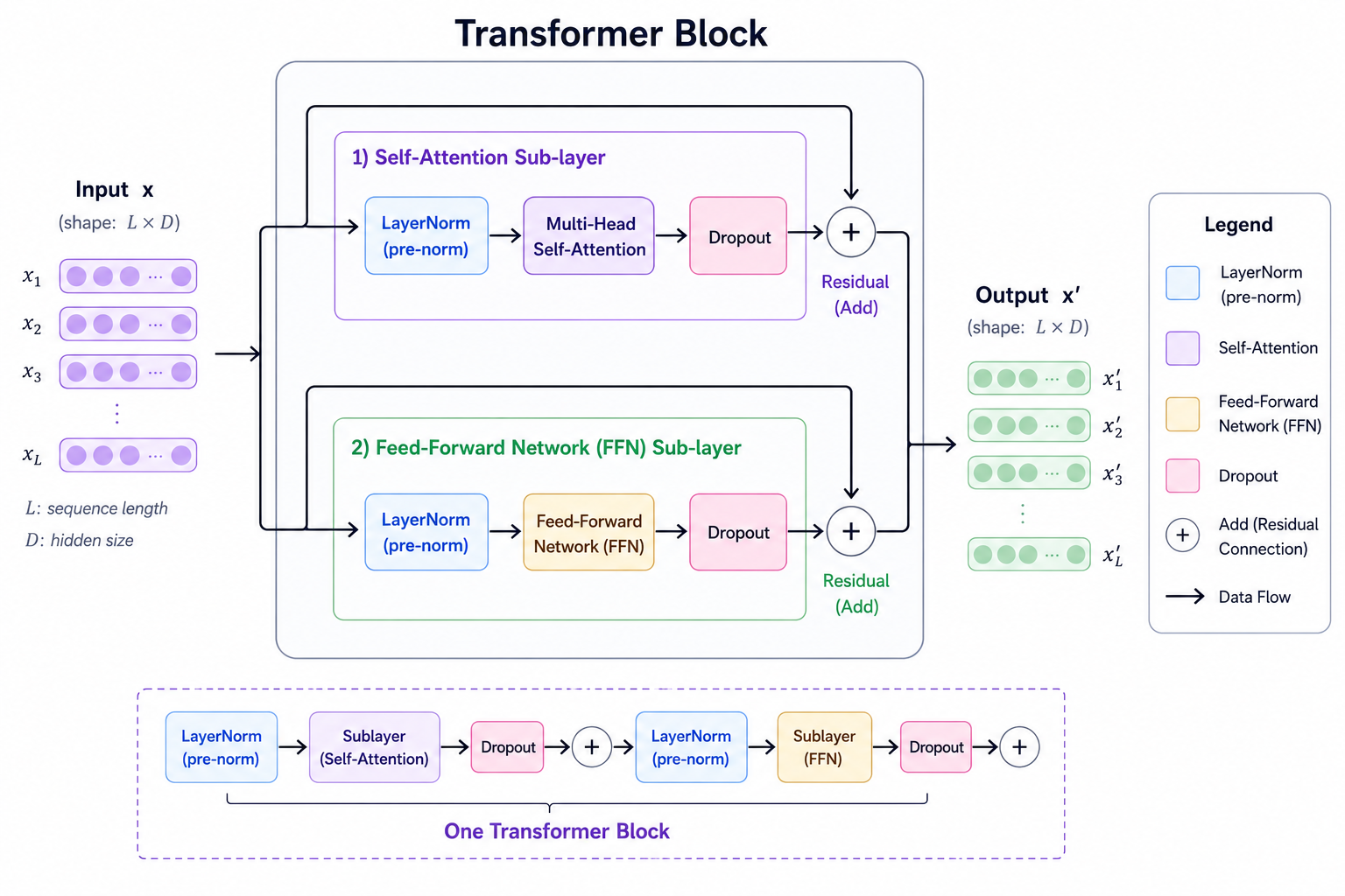 One transformer block: two sub-layers, each wrapped in a pre-norm + residual path
Scaled Dot-Product Attention
The attention mechanism computes, for each position in the sequence, a weighted sum of all other positions. The weights are derived from how similar the current position’s query is to every other position’s key.
Given an input matrix , we compute three projections:
The attention output is:
The scaling prevents the dot products from growing large as dimension increases, which would push softmax into regions with near-zero gradients. is not a free parameter — it’s derived as , where is the number of attention heads. For a model with and , each head has . The scaling factor therefore grows with head dimension, keeping attention scores in a reasonable range regardless of model size.
The result is that each output position is an average of all value vectors, weighted by how much each position’s query “agrees” with each position’s key. Positions that agree strongly get high weights; irrelevant positions get suppressed.
Multi-Head Attention
Running a single attention operation forces the model to represent all relationships in one subspace. Multi-head attention splits the embedding dimension into heads, runs attention independently in each, and concatenates the results:
Each head learns to attend to different types of relationships — syntax, coreference, semantic similarity, positional proximity — simultaneously. A model with and has each head operating in a 64-dimensional subspace.
The Feed-Forward Network
The FFN is applied independently to each position after attention. It expands the representation to a larger dimension, applies a non-linearity, and projects back:
The expansion ratio is typically 4x (so ). This is where most of the model’s “knowledge storage” happens — the attention layers route and mix information, the FFN layers transform it.
Residual Connections and Normalization
Both the attention and FFN sub-layers use residual connections: the input is added back to the sub-layer output before normalization.
The intuition is that each layer learns a small correction rather than a full transformation. Instead of learning to compute the final representation from scratch, the sub-layer only needs to learn what to add to what it already has. In a 96-layer model, 96 small incremental refinements are far easier to optimize than one monolithic transformation. The gradient picture is equally clean: with a residual path, gradients flow directly from the loss back to early layers without passing through every sub-layer in sequence. Without residuals, gradients must traverse every transformation in the chain — in deep networks they vanish before reaching early layers or explode before reaching late ones.
Normalization addresses a different problem: the scale of activations across different positions can vary wildly. A position with large activations would dominate the residual sum; one with small activations would barely contribute. Normalizing each position to a consistent scale before passing it into the sub-layer keeps all positions on equal footing and stabilizes training regardless of depth.
Pre-norm vs. post-norm is a subtle but important distinction. The original transformer applied normalization after the residual addition (post-norm). Modern LLMs apply it before (pre-norm):
Post-norm:  output = LayerNorm(x + Sublayer(x))
Pre-norm:   output = x + Sublayer(LayerNorm(x))
Pre-norm leads to more stable training at scale — this was formalized in “On Layer Normalization in the Transformer Architecture” (Xiong et al., 2020), which showed that post-norm has poorly conditioned gradients at initialization while pre-norm maintains bounded gradient norms throughout. With post-norm, gradients must pass through the normalization layer before reaching the residual path, which can cause instability in very deep networks. Pre-norm keeps the residual path gradient-clean throughout training.
Causal Self-Attention
In a standard transformer encoder, every position can attend to every other position — the attention matrix is fully dense. For language generation, this is a problem: when predicting token , the model cannot have seen tokens
A decoder block enforces this by masking the attention matrix. Future positions are set to before the softmax — and since , those positions receive exactly zero weight after exponentiation. The softmax denominator sums only over the unmasked positions, so the remaining weights still sum to 1. The result is a lower-triangular attention pattern: each position attends only to itself and positions to its left.
Position:   1   2   3   4
         ┌───────────────┐
    1    │ ✓   ✗   ✗   ✗ │
    2    │ ✓   ✓   ✗   ✗ │
    3    │ ✓   ✓   ✓   ✗ │
    4    │ ✓   ✓   ✓   ✓ │
         └───────────────┘
Causal mask: each token attends only to preceding tokens
Key Hyperparameters
A transformer’s size is fully determined by four numbers: (embedding dimension), (number of attention heads), (number of stacked blocks), and (FFN hidden dimension). The total parameter count is approximately:
This formula comes from the four attention projection matrices ( per layer) plus the two FFN matrices ( per layer, assuming ). Two things worth noting: directly changes the 8 coefficient — if a model uses (common with SwiGLU, to compensate for the extra gate matrix), the FFN term is closer to per layer. does not appear in the formula at all — the total Q, K, V parameter count is regardless of how many heads you split them into. More heads means smaller head dimension, not more parameters. It’s a useful number to have memorized — it lets you estimate model size from architecture details and vice versa.
The compute cost of a single forward pass scales as in sequence length — the comes from computing the full attention matrix , and each of those dot products operates over -dimensional vectors. This is the root of most inference and training challenges at long context lengths.
Why Decoder-Only Won
The original transformer had both an encoder and a decoder, designed for sequence-to-sequence tasks like translation. The encoder reads the full input bidirectionally. The decoder generates output autoregressively and has three sub-layers: causal self-attention (attends to previously generated tokens), cross-attention (the K and V projections come from the encoder’s output, while Q comes from the decoder’s own representation — this is how the decoder conditions on the source input), and an FFN. This cross-attention coupling is the architectural reason the encoder and decoder must be trained jointly.
For a long time, the field used different architectures for different tasks: encoder-only (BERT) for understanding tasks, encoder-decoder (T5) for generation tasks, and decoder-only (GPT) for open-ended generation. Then GPT-3 arrived and showed that a large decoder-only model, trained on next-token prediction, could do all of these — and much more.
Why did decoder-only win?
Simplicity at scale. An encoder-decoder model has two components that must be jointly trained, with cross-attention connecting them. A decoder-only model is a single unified component. Simpler architecture means fewer engineering decisions, more stable distributed training, and easier scaling.
The pretraining objective aligns perfectly. Next-token prediction on massive web text trains every parameter of a decoder-only model on every token. In an encoder-decoder model, the encoder receives no direct gradient signal from the language modeling loss — it learns only what the decoder asks it to via cross-attention. The encoder’s parameters must justify their compute budget indirectly, through a bottleneck they don’t control. In a decoder-only model, every layer participates in every prediction, and every token acts as both a context provider and a prediction target. There is no auxiliary component and no wasted capacity.
Emergent generalization. It turned out that a model trained to predict the next token at scale learns representations rich enough to handle tasks it was never explicitly trained on — translation, summarization, reasoning, coding. The causal structure doesn’t limit the model; it shapes it.
Inference simplicity. At inference time, a decoder-only model generates token by token, caching the key-value projections of the prefix to avoid recomputation. An encoder-decoder requires running the encoder once, then running the decoder autoregressively while attending to encoder outputs — two separate inference phases with more complex memory management.
The field didn’t reach this conclusion from first principles — it was empirical. GPT-3 (Brown et al., 2020) showed a 175B decoder-only model could outperform task-specific fine-tuned encoder models on a wide range of tasks. Encoder models kept scaling — RoBERTa, DeBERTa, DeBERTaV3 — but their ceiling became visible: they solved GLUE and SuperGLUE while open-ended generation remained out of reach. The most direct architectural comparison is “What Language Model Architecture and Pretraining Objective Work Best for Zero-Shot Generalization?” (Wang et al., 2022), which tested causal LMs, prefix LMs, and encoder-decoder models at matched parameter counts. Decoder-only with causal language modeling consistently won on zero-shot and few-shot tasks — exactly the setting that matters for a general-purpose assistant.
Interview angle “Why not encoder-decoder for an LLM?” Interviewers are checking whether you understand the tradeoff, not just the outcome. The answer is: decoder-only is simpler, scales better, and the next-token objective turns out to be sufficient for general intelligence at scale. Encoder-decoder is still useful when the input/output lengths differ dramatically or when you need full bidirectional context over a fixed input (e.g. document classification, extractive tasks).
Key Architecture Decisions in Modern LLMs
The vanilla transformer from “Attention Is All You Need” looks quite different from LLaMA or Mistral. Here’s what changed and why each change matters.
Positional Encoding: RoPE and ALiBi
Attention is permutation-invariant — if you shuffle the input tokens, the attention output shuffles identically. Positional information has to be injected explicitly.
The original transformer used fixed sinusoidal embeddings added to the token embeddings before the first layer. This works, but it’s limited: the model sees absolute positions encoded in fixed patterns, and generalizing to lengths longer than those seen during training is difficult.
The deeper problem is that absolute position is the wrong signal. The relationship between two words depends on how far apart they are, not where each sits in the document. “Alice chased her cat” carries the same pronoun-antecedent relationship whether it appears at position 5–9 or position 5005–5009. Absolute encodings force the model to relearn the same dependency at every position — a massive waste of capacity. What the model actually needs is the relative distance between tokens, and that information belongs in the attention computation, not in the embedding.
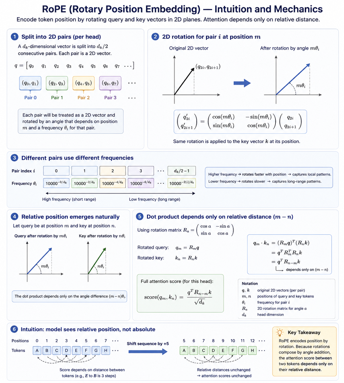
RoPE (Rotary Position Embedding) encodes position directly into the attention mechanism rather than the embeddings. Instead of adding a positional signal to token representations, it rotates the query and key vectors by an angle proportional to their position. The attention score between two tokens then naturally reflects how far apart they are, because the dot product of two rotated vectors depends only on their angular difference.
Concretely, here is what happens step by step. The query vector for a token is computed the normal way: . RoPE then takes this already-computed query vector and applies a position-dependent rotation to it — it does not change the projection weights at all.
The -dimensional query vector is split into consecutive pairs: . Each pair is treated as a 2D vector and rotated by an angle that depends on the token’s position and a frequency assigned to that pair:
Here and are just the -th and -th elements of the query vector — two ordinary floating-point numbers produced by the linear projection. The rotation matrix is the standard 2D rotation: it spins the vector by angle in the plane defined by those two dimensions. The same rotation is applied to the key vector at its own position.
The same process applies to every pair independently, each with its own frequency . The exact same rotation is applied to the key vector at its position. When you then compute , the rotation matrices cancel to yield a term that depends only on :
where is the rotation matrix for offset . The full attention score becomes:
The model never sees absolute position — only relative distance is baked into the computation.
A visual for mental model.
RoPE generalizes better to longer sequences than sinusoidal embeddings, and it can be extended to unseen context lengths (with techniques like YaRN and LongRoPE, covered later). It’s used in LLaMA, Mistral, Qwen, and essentially every modern open-source LLM.
ALiBi (Attention with Linear Biases) takes the opposite philosophy: don’t learn positional representations at all. Instead, subtract a linear penalty from the attention scores based on the distance between tokens:
where is a head-specific slope. Tokens far away get penalized more, making the model implicitly prefer attending to nearby context. ALiBi requires no position embeddings and generalizes well to lengths beyond training — the penalty simply continues growing. It was used in Bloom and MPT. It’s less flexible than RoPE for tasks that require attending to distant tokens, but extremely simple to implement.
Interview angle “What’s the difference between RoPE and ALiBi?” RoPE encodes relative position by rotating Q/K vectors — learned, expressive, requires position-aware projections. ALiBi applies a fixed distance penalty to attention scores — no learning, very simple, good extrapolation. RoPE is dominant today because it’s more expressive and integrates well with extensions like YaRN.
The GQA Spectrum: MHA → GQA → MQA
Standard multi-head attention (MHA) gives each head its own set of key and value projection matrices. For a model with heads, you have sets of Q, K, and V weights.
Before explaining why this is a problem, it’s worth understanding the KV cache — the memory structure that makes autoregressive generation tractable. When generating token , the model must attend to all previous tokens . Rather than recomputing their K and V projections from scratch on every step, we store them after the first computation. The KV cache is this accumulating store of past key and value projections, one entry per token per layer. Without it, generating a 1000-token response would require running 1000 full forward passes over an ever-growing prefix; with it, each step is one forward pass over just the new token. We’ll go much deeper on KV cache mechanics in the inference post — for now, know that it’s the dominant memory consumer during generation.
This becomes a problem at inference time. As you generate a long sequence, the KV cache for every past token in every layer must stay in GPU memory. For a 70B model with 80 layers and 64 heads, the KV cache for a single 8K-token sequence consumes roughly 160GB of GPU memory — more than the model itself.
Multi-Query Attention (MQA) fixes this by sharing a single set of K and V projections across all query heads. Each head has its own Q matrix, but they all read from the same K and V. This reduces the KV cache size by a factor of (from to per token per layer). The downside is a measurable quality drop — all heads are constrained to attend using the same keys and values.
Grouped-Query Attention (GQA) splits the difference. Query heads are divided into groups, and each group shares a K/V head. MHA is (one K/V per query); MQA is (one K/V total); GQA is anything in between.
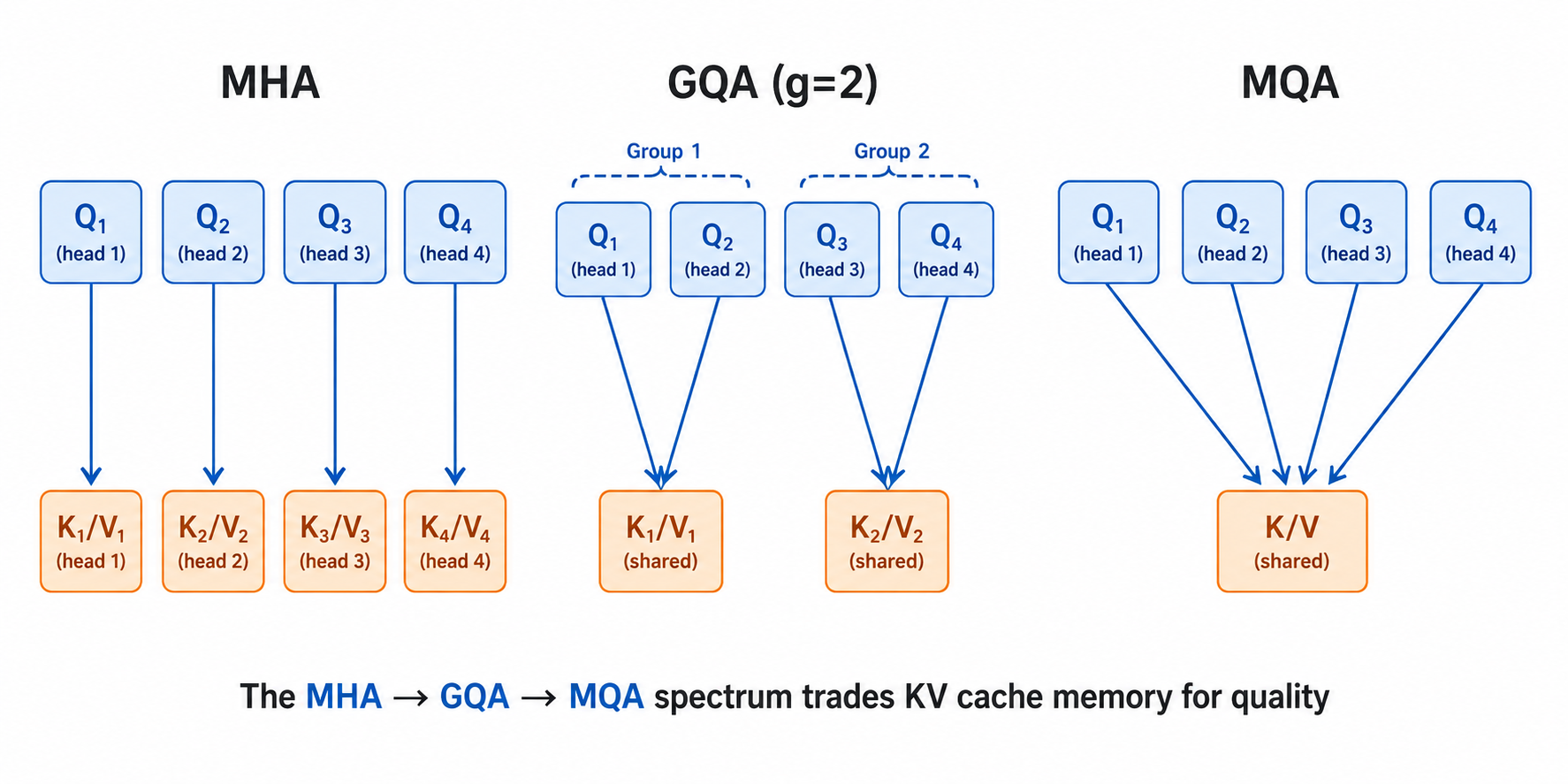 The MHA → GQA → MQA spectrum trades KV cache memory for quality
GQA is the standard choice in modern LLMs. LLaMA 2 70B uses 8 KV heads for 64 query heads (), reducing KV cache by 8× with minimal quality loss. Mistral uses 8 KV heads for 32 query heads. The sweet spot empirically seems to be between 4 and 8.
The memory reduction is straightforward to compute. With MHA, the KV cache per token is bytes (factor of 2 for K and V, ). Since , this simplifies to per token. With GQA using KV heads, the cache becomes . For LLaMA 2 70B in bfloat16 (, , ):
At 8K context that’s ~2.6 GB — compared to ~20 GB with MHA (). The 8× KV head reduction gives exactly 8× cache reduction, which directly translates to 8× more sequences you can hold in memory simultaneously (higher serving throughput).
Flash Attention
Attention has quadratic memory complexity in sequence length. For a sequence of tokens, computing the full attention matrix requires materializing an matrix. At , that’s 67 million floats per head — just for one layer’s intermediate computation.
Flash Attention doesn’t change the mathematical result of attention — it computes the exact same values. What it changes is where the computation happens. Standard attention writes the matrix to GPU HBM (high-bandwidth memory) and reads it back for the softmax and value aggregation. Flash Attention tiles the computation so that it fits in SRAM (on-chip cache), which is orders of magnitude faster to read from.
The trick is a numerically stable online softmax algorithm. Normally, computing requires two passes over all values: one to find the maximum (for numerical stability, to avoid overflow when exponentiating large numbers), and one to compute the normalized exponentials. Flash Attention does this in a single pass by maintaining two running statistics as it tiles through key/value blocks: a running maximum and a running normalization factor . When a new block of attention scores arrives:
The previously accumulated output is rescaled by to account for the updated maximum. At the end of all blocks, you have the correctly normalized softmax output without ever materializing the full matrix. Each tile of Q and K fits in SRAM, computation happens there, and only the final accumulated output is written back to HBM.
Standard attention:
  Write QKᵀ to HBM (slow) → Read for softmax (slow) → Write result → Read for ×V (slow)

Flash Attention:
  Tile: load Q block + K block into SRAM → compute partial attention in SRAM → accumulate result
  Never write the full n×n matrix to HBM
Flash Attention reduces memory from to while running 2–4× faster on A100s.
Flash Attention 2 addressed a parallelism bottleneck in the original. FA1 parallelized across batch size and attention heads — each (batch, head) pair was processed by one thread block. For long-sequence, small-batch workloads (common in inference), this left GPU utilization low: if you have batch size 1 and 32 heads, only 32 thread blocks run in parallel, leaving most SMs idle. FA2 added parallelism across the sequence dimension — it splits the query sequence into chunks and processes each chunk independently, so the number of thread blocks scales with sequence length rather than being capped at batch × heads. FA2 also improved work partitioning within each thread block, reducing wasted warp cycles. Together these changes gave another 2× speedup over FA1.
Flash Attention 3 targets H100-specific features: FP8 tensor core utilization, asynchronous data movement between HBM and SRAM, and better pipelining of matrix multiply and softmax stages. Every production LLM training and serving system uses Flash Attention.
Interview angle “What does Flash Attention actually do?” The key is “IO-aware” — it doesn’t change the math, it changes where the computation happens. Keeping it in SRAM instead of writing to HBM eliminates the bandwidth bottleneck. This is the same insight that drives kernel fusion in general: memory bandwidth, not FLOPs, is usually the limiting factor.
RMSNorm
The original transformer used Layer Normalization, which normalizes activations by subtracting the mean and dividing by the standard deviation, then applying a learned scale and shift.
Modern LLMs use RMSNorm (Root Mean Square Normalization), which drops the mean-centering step and only normalizes by the RMS of the activations:
Why? Empirically, the mean-centering in LayerNorm contributes little to training stability while adding compute cost. RMSNorm is faster (fewer operations), and at the scale of billions of parameters, this matters. It’s also more numerically stable in mixed-precision training. RMSNorm was introduced in “Root Mean Square Layer Normalization” (Zhang & Sennrich, 2019) and is now the default normalization in every major open LLM: LLaMA 1/2/3, Mistral, Falcon, Qwen, PaLM, Gemma.
SwiGLU Activation
The standard FFN uses ReLU or GELU activations. Modern LLMs use SwiGLU, a gated linear unit variant:
The intuition for why this is better than a standard activation: ReLU and GELU apply the same nonlinearity uniformly to every feature of the FFN input. SwiGLU introduces a learned gate — the term — that lets the network decide independently for each feature how much of the transformation to let through. When the gate is near 0, that feature is suppressed; when it’s near 1, it passes through at full magnitude. This gives the FFN finer-grained control over which features to transform and which to ignore, which translates to better loss at the same parameter count.
The cost is a third weight matrix. A standard FFN uses and — two matrices. SwiGLU needs an additional for the gate path. To keep total parameter count equal to a standard FFN with , you solve , giving . This is exactly the expansion ratio used in LLaMA models. The original comparison and the rule come from Noam Shazeer’s “GLU Variants Improve Transformer” (2020).
Mixture of Experts
All the architecture decisions above apply to dense models — every token activates every parameter on every forward pass. Mixture of Experts (MoE) breaks this assumption.
In a MoE layer, the FFN is replaced with multiple “expert” FFNs (typically 8 or more). A small router network looks at each token’s representation and picks the top- experts (usually ) to process it. The outputs of the selected experts are weighted and summed.
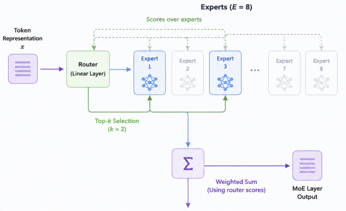
The key insight is that a model with 8 experts of size has 8× the parameter count of a dense model, but only activates 2× the FFN compute per token. You get the representational capacity of a large model at the compute cost of a smaller one. Mixtral 8×7B has 47B parameters but uses only ~13B active parameters per token — matching or beating LLaMA 2 13B quality at similar inference cost.
How the Router Works
The router is a small linear layer , where is the number of experts. For each token representation , it computes a score over all experts:
The top- experts (typically ) are selected, and the token is processed independently by each. The outputs are combined as a weighted sum using the router scores:
The renormalization over selected experts (not all experts) ensures the output weights sum to 1.
Memory: All Experts Must Be Loaded
A common misconception: MoE does not reduce memory at inference — it increases it. All expert FFNs must reside in GPU memory simultaneously, because you don’t know which expert will be activated until you’ve run the router for each token. A Mixtral 8×7B model has 47B parameters total, and all 47B must be loaded. What MoE saves is compute per token, not memory. This distinction matters enormously for deployment: MoE models need more GPUs than their active-parameter count suggests, because all experts must fit in VRAM.
For DeepSeek-V3 (671B parameters total, ~37B active), the entire 671B parameter set must be distributed across GPUs using expert parallelism — each GPU holds a subset of experts. At inference time, tokens are routed across GPUs via all-to-all communication, processed by the appropriate expert, and results aggregated.
Gradient Flow Through Non-Activated Experts
Gradient does not flow through non-activated experts for a given token — if Expert 3 wasn’t selected for token , Expert 3’s weights receive no gradient from ‘s prediction. This is by design: the router makes a discrete selection, and the straight-through estimator (treating the selection as differentiable) isn’t used here. Instead, gradients only flow through the selected experts.
This means each expert gets gradient from only a fraction of tokens per batch. If load balancing works correctly, each expert sees roughly of all tokens — for , , each expert is updated on ~25% of tokens per batch. With large enough batch sizes, this is sufficient.
Expert Collapse and Load Balancing
The failure mode during training is expert collapse: the router gravitates toward a small set of experts and stops sending tokens to the rest. Once an expert receives fewer tokens, it gets less gradient, its weights don’t improve, and the router learns to avoid it further — a vicious cycle that leaves most of the model’s capacity unused.
Two mechanisms prevent this:
Auxiliary load-balancing loss. An auxiliary term penalizes the variance in expert utilization across a batch. If expert 1 receives 60% of tokens and expert 8 receives 2%, the auxiliary loss fires heavily. This loss is added to the main training objective with a small coefficient (typically ).
Expert capacity limits. Each expert has a maximum number of tokens it can process per batch (the capacity factor, typically 1.0–1.25× the average expected load). Tokens routed to an overloaded expert are either dropped (processed via the residual connection without FFN transformation) or redirected to a backup expert. This hard cap forces tokens to distribute even if the router has a soft preference.
DeepSeek-V3 took a different approach: instead of an auxiliary loss (which can interfere with the main training objective), it adds a small learnable bias to each expert’s router score that shifts traffic away from overloaded experts during training. This auxiliary-loss-free load balancing achieved better model quality by not polluting the gradient signal with a secondary objective.
Training and Inference Optimizations
Expert parallelism is the key distributed strategy. Experts are sharded across GPUs — each GPU owns a subset. The attention layers run normally, but at the FFN (MoE) layer, tokens must be dispatched to the correct GPU based on the router’s decision. This requires an all-to-all communication collective: each GPU sends tokens assigned to remote experts and receives tokens assigned to its local experts. After FFN computation, another all-to-all routes results back. This communication cost is the main overhead of MoE training and inference.
At inference, small batch sizes (common in serving) hurt MoE utilization. With batch size 1 and top-2 out of 8 experts, only 2 experts are active and 6 GPUs sit idle (if experts are on separate GPUs). This is why MoE is often better suited for training throughput than low-latency serving. Larger batch sizes amortize the per-request expert-switching cost — a batch of 64 requests will likely activate most experts in each layer.
Interview angle “When would you choose MoE over a dense model?” MoE wins when you have a fixed inference budget but want higher model capacity — you need the intelligence of a large model but can’t afford its compute per token. The cost is more complex training (load balancing), higher total memory (all experts must be loaded), and trickier distributed inference. DeepSeek-V3 (685B params, ~37B active) shows this scaling to extreme sizes.
Long Context Techniques
The quadratic attention complexity means context length has always been a bottleneck. Modern LLMs support 128K–1M token contexts through a combination of architecture changes and training techniques.
Extending RoPE
To understand context extension, you first need a concrete picture of what RoPE actually does to each dimension of the Q/K vectors.
Recall that RoPE splits the head dimension into pairs. For a head with , you get 32 pairs: . Each pair is rotated by an angle that depends on the token’s position — but crucially, each pair gets its own rotation speed, called its rotation frequency:
Pair 0 () uses radian per position. Pair 31 () uses radians per position. The frequencies decrease exponentially as grows, spanning four orders of magnitude.
In concrete terms for a 4K training context:
- Pair 0 (fastest): At position 4096, this pair has rotated radians — about 652 full rotations.
- Pair 31 (slowest): At position 4096, this pair has rotated radians — not even a tenth of a full rotation.
The fast-rotating pairs are sensitive to small position differences — two tokens 3 apart have very different angles in pair 0. The slow-rotating pairs stay distinguishable across long spans — two tokens 10,000 apart still have different angles in pair 31.
Now here’s the problem when you try to extend from 4K to 128K context without any changes. The fast pairs are fine: at position 128K, pair 0 has rotated radians. The model has seen pair 0 complete hundreds of full rotations during training, and two nearby tokens still have a small relative angle. The fast pairs generalize.
The slow pairs break. During training, pair 31 reached a maximum angle of 0.55 radians. At position 128K, pair 31 would reach radians. The model has never seen pair 31 with an angle above 0.55 rad — so 17.3 rad is completely out-of-distribution. Attention scores computed using these dimensions become unreliable.
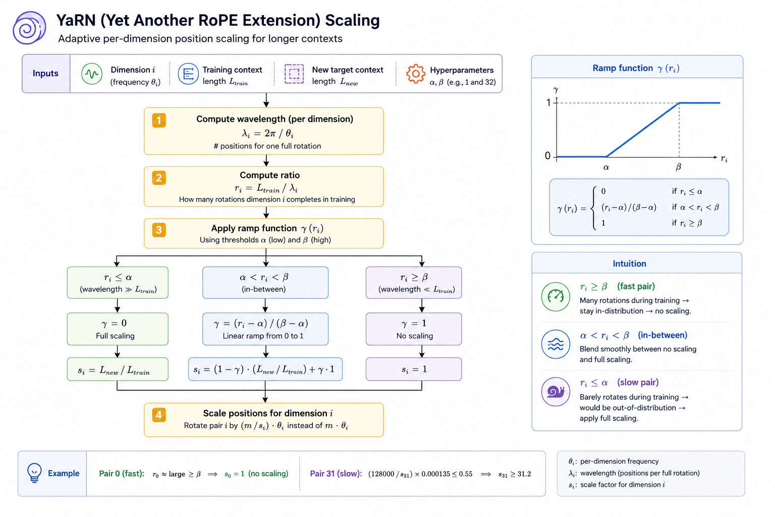
YaRN (Yet Another RoPE Extension) fixes this by rescaling positions differently for each pair. Instead of rotating pair at position by , it rotates by , where is a per-dimension scale factor. For pair 31 with target context 128K, you want:
For pair 0 (fast, already fine), — no scaling needed. YaRN applies aggressive scaling to the slow pairs and leaves the fast pairs alone, with a smooth interpolation in between. This keeps all dimension pairs within the angle range the model trained on, regardless of how long the context is.
The decision rule is based on each dimension’s wavelength: — the number of positions needed to complete one full rotation. Pair 0 has positions; pair 31 has positions.
YaRN formalizes the scaling decision using a ramp function defined over the ratio — how many full rotations pair completes within the training context. Two thresholds, and (hyperparameters, set to 1 and 32 in the paper), split all dimensions into three regions:
- (wavelength much shorter than , fast pair): the dimension completed many cycles during training. , so — no scaling.
- (wavelength much longer than , slow pair): the dimension barely rotated during training and will go far out-of-distribution. , so — full scaling.
- : ramps linearly from 0 to 1, blending between full scaling and no scaling. The effective scale is .
Every dimension gets its own from this formula — no per-model manual tuning, just two boundary hyperparameters and the ratio of the two context lengths.
YaRN still requires brief fine-tuning — you cannot simply change the scaling at inference time without retraining. The attention patterns learned during pretraining were calibrated to the original angle distribution. Fine-tuning for a few hundred steps on long-context data (at the target length) updates these patterns cheaply — far cheaper than pretraining from scratch.
LongRoPE takes the same idea but replaces YaRN’s hand-designed scaling formula with an automated search. It maintains a population of candidate scaling vectors — each vector specifies one scale factor per RoPE dimension pair. At each generation, candidates are evaluated by running the model on long-context validation data and measuring perplexity. The best-performing candidates are kept, the rest are replaced with combinations and perturbations of the survivors. This is evolutionary search: no gradients, just a survival-of-the-fittest loop over candidate configurations. After many generations, the search converges on near-optimal per-dimension scaling. The result beats YaRN’s formula, at the cost of significant search compute. Both methods allow extending a 4K model to 128K context with a fraction of the compute of full pretraining.
Attention Patterns for Long Context
Even with extended RoPE, attention over 128K tokens is expensive. Several architectures modify the attention pattern to reduce this cost.
Sliding window attention restricts each token to attending only to the most recent tokens, reducing attention complexity from to . Mistral uses a window of 4096 tokens within its 32K context window. This seems to cut off long-range dependencies — but in a multi-layer model, it doesn’t. With window size and layers, a token at layer has an effective receptive field of tokens, because information from distant past tokens propagates through intermediate tokens layer by layer. A 32-layer model with has an effective receptive field of 131K tokens — the long-range context is captured indirectly through the chain of layers.
The tradeoff is that very specific long-range recall (e.g., remembering a fact mentioned 50K tokens ago verbatim) degrades, because information must pass through many lossy intermediate representations rather than being accessed directly. For tasks where any-token-to-any-token attention matters, sliding window alone is insufficient.
Sparse attention (as in Longformer and BigBird) addresses this by combining a local window with a small set of global tokens. The pattern has three components: every token attends to a local window of size around it; a designated set of global tokens (e.g., a [CLS] token or the first few tokens) attends to every other token and is attended to by every other token; and optionally, some random token pairs get attention links. The global tokens act as aggregation points — local tokens funnel information to them through the local window, and the global tokens broadcast that information back to the whole sequence. This gives every token indirect access to the full context in steps via the global tokens, without the cost of full attention.
The “Lost in the Middle” Problem
Even when long contexts work technically, LLMs perform better when relevant information appears at the beginning or end of the context rather than the middle. Performance degrades for information buried in the middle of a long sequence — a well-documented phenomenon called “lost in the middle.”
The practical implication for system design: when building RAG or long-document systems, place the most critical information at the start or end of the context. This isn’t a flaw being fixed — it’s an architectural property to design around.
Architectural Evolution at a Glance
The jump from the original transformer to modern LLMs involves a consistent set of changes across all architectures:
| Component | Original Transformer | Modern LLM (e.g. LLaMA 3) |
|---|---|---|
| Normalization | Post-norm, LayerNorm | Pre-norm, RMSNorm |
| Position | Sinusoidal embeddings | RoPE |
| Attention | MHA | GQA |
| FFN activation | ReLU | SwiGLU |
| Attention compute | Standard | Flash Attention |
| Architecture type | Encoder-Decoder | Decoder-only |
Each change was driven by empirical evidence at scale — not theory. Pre-norm stabilizes training. RoPE generalizes better. GQA cuts KV cache. SwiGLU improves loss. Flash Attention enables long context. None of these is a dramatic conceptual shift; together they make the difference between a model that works at 1B parameters and one that scales to 400B.
Mental Model
A transformer is a function that maps a sequence of vectors to a sequence of vectors. Each block refines the representations by letting every position gather information from all other positions (attention) and then transform its own representation nonlinearly (FFN). Stack enough blocks and train with enough data, and the representations become rich enough to encode grammar, facts, reasoning, and style. The decoder-only variant simply restricts attention to past tokens, which makes it naturally suited to autoregressive generation. All the modern improvements — RoPE, GQA, RMSNorm, SwiGLU, Flash Attention — are engineering choices that make this architecture stable, memory-efficient, and fast at scale. Understanding why each exists is what separates a strong interview candidate from one who can only recite the name.
Further Reading
- Attention Is All You Need — the original transformer paper
- RoFormer: Enhanced Transformer with Rotary Position Embedding — RoPE
- GQA: Training Generalized Multi-Query Transformer Models — GQA
- FlashAttention-2: Faster Attention with Better Parallelism and Work Partitioning — Flash Attention 2
- Mixtral of Experts — MoE at scale