In post 1.4 we ran gradient descent on a single training example and watched the weight converge to the right answer in a few steps. But that assumed we were computing the exact gradient over the entire dataset before each update. That breaks down as soon as the dataset gets large. This post covers how we fix that - and then how we make training smarter, not just faster.
Why it exists
Imagine your training set has 10 million images. Basic gradient descent computes the gradient over all 10 million samples and then updates the weights once. That’s 10 million forward passes per step. Training would take weeks before weights move at all.
The obvious fix: don’t use the full dataset. Pick a random subset of, say, 64 samples, compute the gradient on those, update the weights, then pick another 64. Each update is noisier than the true gradient, but the weights still converge on average - and you make thousands of updates in the time one full-dataset step would take.
This is SGD (Stochastic Gradient Descent). “Stochastic” means random. The random subset is called a mini-batch. In practice, “SGD” almost always means mini-batch SGD - nobody uses single-sample updates or full-dataset updates.
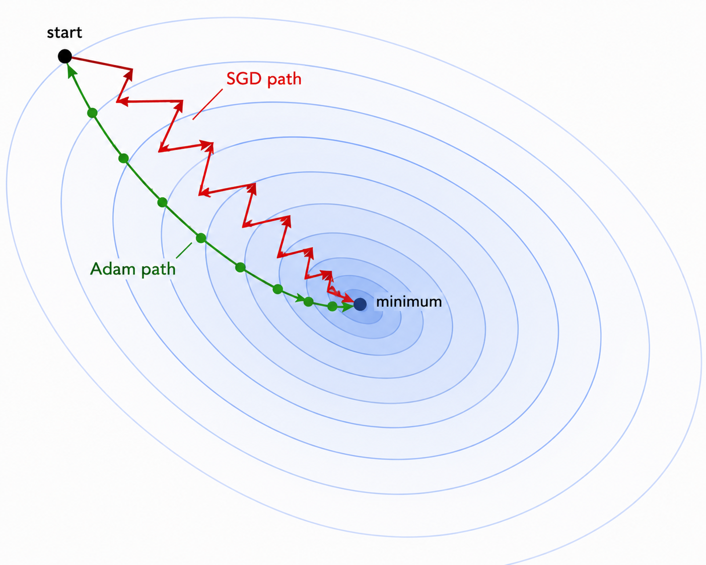
SGD is fast. But it has a problem: it zigzags. On a loss landscape that is steep in one direction and flat in another, each gradient step overshoots across the steep direction while barely advancing in the flat one. You waste updates bouncing back and forth. The rest of this post is about fixing that.
How it works
Momentum
Momentum adds memory to SGD. Instead of using the raw gradient at each step, you keep a velocity - a running average of past gradients - and update weights using that.
velocity = momentum × velocity + gradient
weight   = weight - lr × velocity
If gradients have been pointing in the same direction for several steps, the velocity builds up and you move faster - like a ball rolling downhill that picks up speed. If gradients keep flipping direction, they cancel out in the average and the velocity stays small - the zigzag dampens.
A typical momentum value is 0.9. That means 90% of the previous velocity carries forward and 10% comes from the current gradient.
This is the same idea as exponential moving average in a monitoring system - you smooth out noise by blending old values with new ones, so spikes don’t dominate your signal.
Adam
Adam (Adaptive Moment Estimation) goes further. It maintains two running averages per parameter:
- 1st moment (m): a running average of gradients - like momentum, smooths the update direction
- 2nd moment (v): a running average of squared gradients - tracks how noisy each parameter’s gradient is
Adam then scales each weight’s step by the inverse of its gradient noise. Parameters with large, consistent gradients get a smaller effective learning rate to avoid overshooting. Parameters with small or infrequent gradients get a larger effective learning rate to still make progress.
m = β1 × m + (1 - β1) × grad        # smoothed gradient
v = β2 × v + (1 - β2) × grad²       # smoothed squared gradient
weight = weight - lr × m / (√v + ε)
Defaults that work across most tasks: β1=0.9, β2=0.999, ε=1e-8, lr=1e-3.
Think of it as each parameter getting its own learning rate that adjusts based on its history - not one global dial for all weights, but an auto-tuned dial per variable. Parameters that rarely get large gradients (say, a less-used embedding) can still learn quickly; parameters that are updated heavily every step won’t overshoot.
Adam converges much faster than SGD in practice, especially early in training. The tradeoff: it uses more memory. Two extra tensors per parameter (m and v) instead of none.
AdamW
AdamW is Adam with one fix: weight decay done correctly.
Weight decay adds a small penalty for large weights at each update step. The intuition is that smaller weights represent simpler functions, which tend to generalise better to data the model hasn’t seen.
In vanilla Adam, weight decay is typically implemented by adding it to the gradient before the update. The problem: that gradient then gets scaled by the adaptive learning rate from the 2nd moment. Parameters with noisy gradients end up receiving less regularisation than parameters with clean gradients - an unintended side effect.
AdamW separates weight decay from the gradient update entirely:
weight = weight - lr × m / (√v + ε) - lr × λ × weightThe second term (- lr × λ × weight) shrinks every weight slightly each step, regardless of the gradient. This is how L2 regularisation is supposed to work - decoupled from the adaptive step.
AdamW is the standard optimizer for LLMs. GPT-2, GPT-3, LLaMA, Mistral - all trained with AdamW.
When to use what
| Optimizer | Use when |
|---|---|
| SGD + momentum | Image models (CNNs). A well-tuned SGD can match Adam with the right schedule |
| Adam | Default for most deep learning - fast convergence, low tuning effort |
| AdamW | Transformers and LLMs. Same as Adam but weight decay works correctly |
The practical default: AdamW with lr=1e-3 for training from scratch, and lr=1e-5 to 5e-5 when fine-tuning a pre-trained model. Lower because pre-trained weights are already good - you want gentle updates, not large steps that overwrite what the model already learned.
Code
Step 1 - train a small network with three optimizers and compare convergence:
Task: fit y = sin(2πx) using a 2-layer network. Nonlinear enough that the optimizer choice matters.
import torch
import torch.nn as nn

torch.manual_seed(42)
X = torch.linspace(0, 1, 200).unsqueeze(1)
y = torch.sin(2 * 3.14159 * X) + 0.1 * torch.randn_like(X)

def make_model():
    return nn.Sequential(
        nn.Linear(1, 32), nn.ReLU(),
        nn.Linear(32, 32), nn.ReLU(),
        nn.Linear(32, 1),
    )

torch.manual_seed(7)
m_sgd    = make_model()
m_sgdmom = make_model()
m_adam   = make_model()
# same starting weights for all three
for p1, p2 in zip(m_sgd.parameters(), m_sgdmom.parameters()):
    p2.data = p1.data.clone()
for p1, p2 in zip(m_sgd.parameters(), m_adam.parameters()):
    p2.data = p1.data.clone()

configs = [
    ("SGD (no momentum)", m_sgd,    torch.optim.SGD(m_sgd.parameters(),    lr=0.01)),
    ("SGD + momentum",    m_sgdmom, torch.optim.SGD(m_sgdmom.parameters(), lr=0.01, momentum=0.9)),
    ("Adam",              m_adam,   torch.optim.Adam(m_adam.parameters(),  lr=1e-2)),
]
loss_fn = nn.MSELoss()
all_losses = {name: [] for name, _, _ in configs}

for _ in range(300):
    for name, model, opt in configs:
        pred = model(X)
        loss = loss_fn(pred, y)
        opt.zero_grad(); loss.backward(); opt.step()
        all_losses[name].append(loss.item())

for name, losses in all_losses.items():
    print(f"{name:25s}  step20={losses[19]:.3f}  step100={losses[99]:.3f}  final={losses[-1]:.3f}")
SGD (no momentum) step20=0.480 step100=0.419 final=0.231
SGD + momentum step20=0.415 step100=0.148 final=0.089
Adam step20=0.177 step100=0.023 final=0.009Momentum cuts the final loss by more than half compared to plain SGD. Adam converges 25x lower by the end.
Step 2 - plot the convergence curves:
import matplotlib.pyplot as plt

fig, ax = plt.subplots(figsize=(8, 4))
colors = ["#94a3b8", "#3b82f6", "#f59e0b"]
for (name, losses), color in zip(all_losses.items(), colors):
    ax.plot(losses, label=name, linewidth=2, color=color)

ax.set_xlabel("Training step")
ax.set_ylabel("Loss")
ax.set_title("SGD vs Momentum vs Adam - convergence speed")
ax.legend()
ax.spines["top"].set_visible(False)
ax.spines["right"].set_visible(False)
plt.tight_layout()
plt.savefig("assets/images/1.5/sgd-vs-adam-loss.png", dpi=150)
plt.show()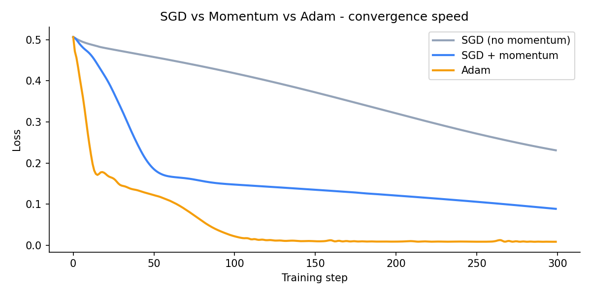
Step 3 - AdamW for fine-tuning a pre-trained model:
import torch

# typical AdamW config when fine-tuning a pre-trained transformer
optimizer = torch.optim.AdamW(
    model.parameters(),
    lr=2e-5,           # lower than default - pre-trained weights need gentle nudges
    weight_decay=0.01,
    betas=(0.9, 0.999),
    eps=1e-8,
)
The only change from Adam: weight_decay=0.01 is applied directly to the weights, not folded into the gradient. Everything else is the same as Adam.
Key takeaways
- SGD uses random mini-batches to make training fast; momentum smooths the update direction by blending past gradients with the current one
- Adam adapts the learning rate per parameter based on gradient history - parameters that rarely update get bigger steps, parameters with large noisy gradients get smaller ones
- AdamW is Adam with weight decay applied separately from the gradient update - the standard choice for training and fine-tuning LLMs
What to read next
Training is now stable and fast - but as data flows through many layers, the values can drift: activations explode or shrink, and training becomes unstable. Normalisation fixes that by keeping each layer’s outputs on a consistent scale.
→ Post 1.6 - Normalisation: BatchNorm and LayerNorm