Gradient Descent and Backpropagation: How a Network Actually Learns

In post 1.1 we said the network learns by adjusting its weights. In post 1.3 we built a way to measure how wrong those weights are. This post connects the two - how do we actually use the loss to fix the weights?

Before we get there, a quick note on training paradigms. Post 1.1 introduced supervised learning - learning from labelled examples. There are two others worth knowing: unsupervised learning, where the model finds patterns in data with no labels (used in clustering and dimensionality reduction); and self-supervised learning, where the model generates its own labels from the data - like predicting the next word in a sentence. Self-supervised learning is how LLMs are pre-trained, covered in Section 4.

Why it exists

We have a network with random weights and a loss function that tells us how wrong it is. The goal is to find the weights that make the loss as small as possible.

One approach: try all possible weight combinations. That’s not feasible - a small network with a million parameters would require more combinations than atoms in the universe.

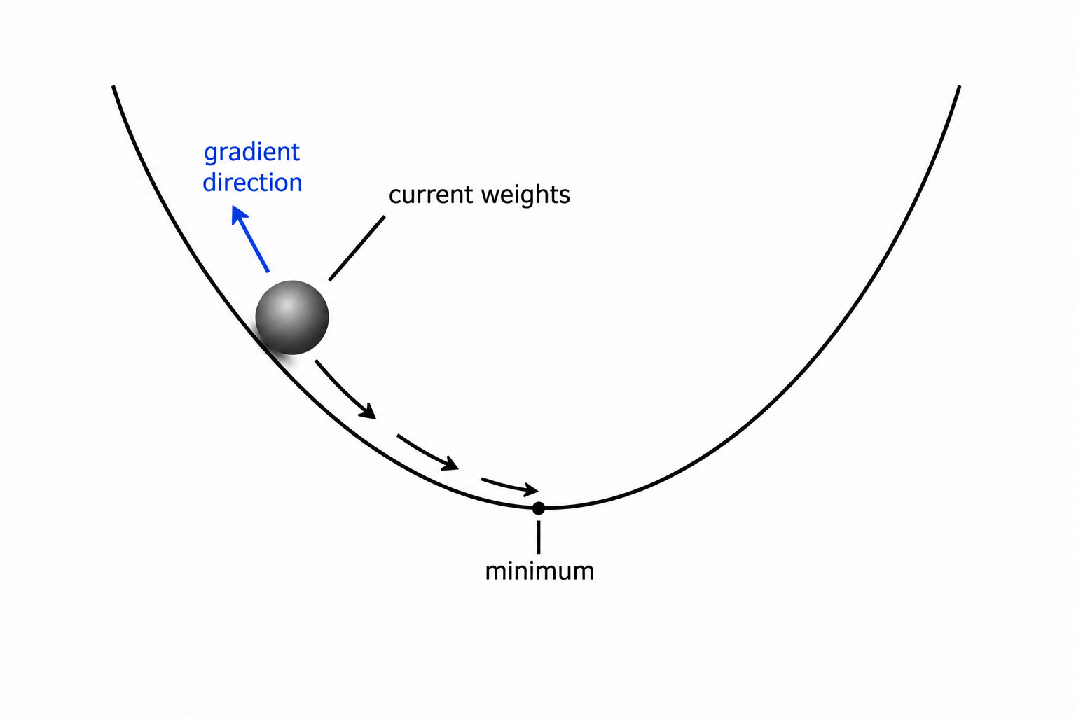
A smarter approach: look at the loss right now, figure out which direction to nudge each weight to make it smaller, and take a small step in that direction. Repeat. This is gradient descent.

How it works

Gradients

A gradient is the derivative of the loss with respect to a weight. It tells you: if I increase this weight by a tiny amount, does the loss go up or down, and by how much?

If the gradient is positive, increasing the weight increases the loss - so we should decrease it. If it’s negative, we should increase it. We always move in the direction opposite to the gradient - downhill on the loss curve.

For a network with millions of weights, we need a gradient for every single one. Computing all of them by hand is impossible. That’s what backpropagation is for.

Gradient descent

The weight update rule is:

weight = weight - learning_rate × gradient

Learning rate controls the step size. Too large and you overshoot the minimum - the loss bounces around or even grows. Too small and training takes forever. A typical starting value is 0.01 or 0.001.

Think of it like a binary search - you keep halving your search space, moving toward the region of lowest loss. Except here you’re following the slope rather than halving, but the intuition is the same: each step gets you closer to the answer.

Backpropagation

Backpropagation (backprop) is the algorithm that computes the gradient of the loss with respect to every weight in the network efficiently.

The key insight is the chain rule from calculus. The network is a composition of functions: loss = L(layer3(layer2(layer1(x)))). The chain rule says the derivative of a composed function is the product of the derivatives of each part:

d(loss)/d(weight_1) = d(loss)/d(layer3) × d(layer3)/d(layer2) × d(layer2)/d(layer1) × d(layer1)/d(weight_1)

Backprop starts at the loss, computes its gradient with respect to the last layer’s output, then works backwards layer by layer - each layer receives the gradient from the layer ahead of it, multiplies by its own local gradient, and passes it further back. Like a traceback in a debugger that propagates error information from the crash site back to the root cause.

PyTorch does all of this automatically. When you call loss.backward(), it traverses the computation graph backwards and fills in the .grad attribute on every tensor that was involved.

One full training step

Every training step follows this exact sequence:

1. Forward pass - feed input through the network, get a prediction
2. Compute loss - measure how wrong the prediction is
3. Backward pass - run backprop, compute gradients for every weight
4. Weight update - nudge each weight in the direction that reduces loss
5. Repeat

Code

Step 1 - gradient descent by hand on a trivial problem:

We want to learn the weight w in y = w × x, given pairs of (x, y). Start with a random w and update it step by step.

# true relationship: y = 3x
# we want the network to discover w = 3

x, y_true = 2.0, 6.0
w = 0.0          # start with wrong weight
lr = 0.1         # learning rate

for step in range(10):
    y_pred = w * x                    # forward pass
    loss   = (y_pred - y_true) ** 2  # MSE loss
    grad   = 2 * (y_pred - y_true) * x  # derivative of loss w.r.t. w
    w      = w - lr * grad            # weight update
    print(f"step {step+1}: w={w:.4f}, loss={loss:.4f}")

step 1:  w=2.4000, loss=36.0000
step 2:  w=2.8800, loss=5.7600
step 3:  w=3.0240, loss=0.9216
step 4:  w=2.9952, loss=0.1475
step 5:  w=3.0010, loss=0.0236
step 6:  w=2.9998, loss=0.0038
step 7:  w=3.0000, loss=0.0006
step 8:  w=3.0000, loss=0.0001
step 9:  w=3.0000, loss=0.0000
step 10: w=3.0000, loss=0.0000

The weight starts at 0 and converges to 3 - the correct value - in a few steps. Loss drops sharply at first and levels off as the weight gets closer to the correct value.

Step 2 - the same thing using PyTorch autograd:

import torch

x, y_true = torch.tensor(2.0), torch.tensor(6.0)
w  = torch.tensor(0.0, requires_grad=True)  # tell PyTorch to track this
lr = 0.1

for step in range(5):
    y_pred = w * x
    loss   = (y_pred - y_true) ** 2

    loss.backward()          # compute gradients automatically

    with torch.no_grad():
        w -= lr * w.grad     # update weight
    w.grad.zero_()           # reset gradient for next step

    print(f"step {step+1}: w={w.item():.4f}, loss={loss.item():.4f}")

step 1: w=2.4000, loss=36.0000
step 2: w=2.8800, loss=5.7600
step 3: w=3.0240, loss=0.9216
step 4: w=2.9952, loss=0.1475
step 5: w=3.0010, loss=0.0236

requires_grad=True tells PyTorch to track operations on w. After loss.backward(), w.grad holds exactly the gradient we computed by hand in step 1. w.grad.zero_() clears the gradient after each update - without this, PyTorch accumulates gradients across steps.

Step 3 - plot the weight converging:

import matplotlib.pyplot as plt
import torch

x, y_true = torch.tensor(2.0), torch.tensor(6.0)
w  = torch.tensor(0.0, requires_grad=True)
lr = 0.1

weights, losses = [], []

for _ in range(15):
    y_pred = w * x
    loss   = (y_pred - y_true) ** 2
    loss.backward()
    weights.append(w.item())
    losses.append(loss.item())
    with torch.no_grad():
        w -= lr * w.grad
    w.grad.zero_()

fig, (ax1, ax2) = plt.subplots(1, 2, figsize=(10, 4))

ax1.plot(weights, marker="o", markersize=4)
ax1.axhline(3.0, color="red", linestyle="--", label="true w=3")
ax1.set_title("Weight over training steps")
ax1.set_xlabel("Step")
ax1.set_ylabel("w")
ax1.legend()

ax2.plot(losses, marker="o", markersize=4, color="orange")
ax2.set_title("Loss over training steps")
ax2.set_xlabel("Step")
ax2.set_ylabel("Loss")

for ax in (ax1, ax2):
    ax.spines["top"].set_visible(False)
    ax.spines["right"].set_visible(False)

plt.tight_layout()
plt.savefig("assets/images/1.4/weight-convergence.png", dpi=150)
plt.show()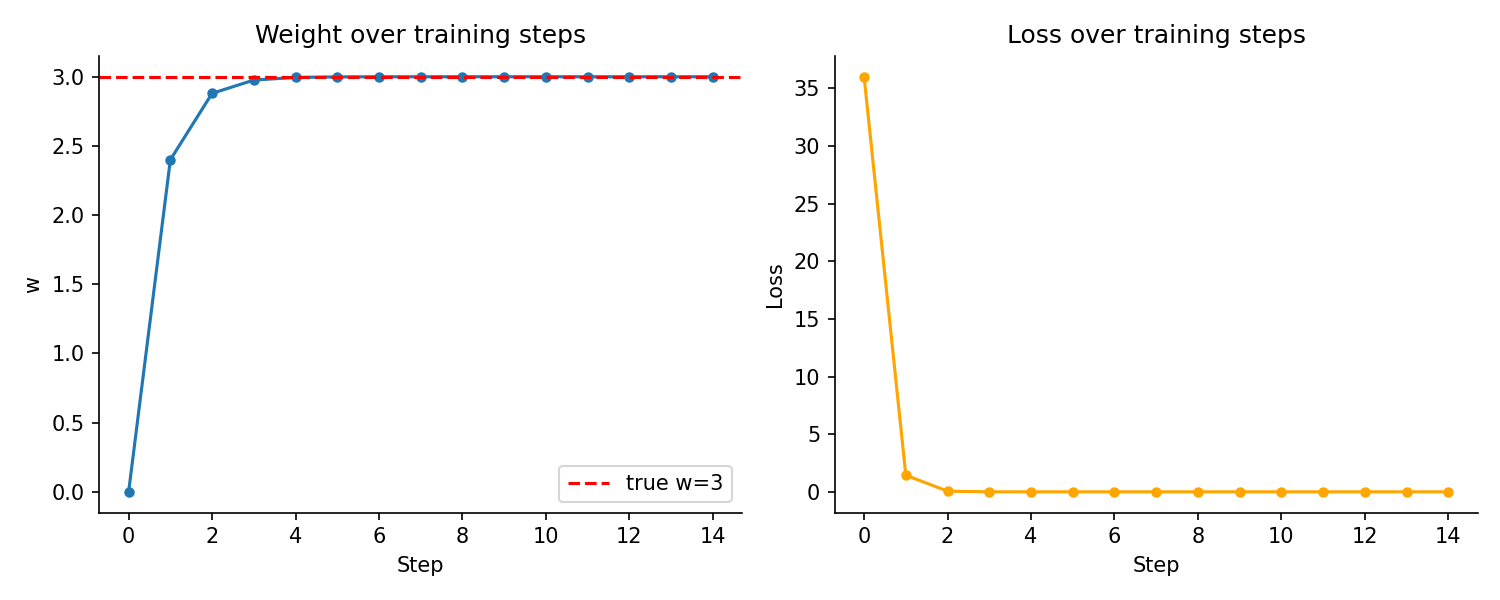

Key takeaways

• A gradient points in the direction that increases the loss - gradient descent moves each weight the opposite way, by a step size controlled by the learning rate
• Backpropagation computes all gradients efficiently using the chain rule, working backwards from the loss through each layer
• One training step = forward pass → loss → backprop → weight update. Repeat thousands of times.

What to read next

Gradient descent works, but the basic version is slow - it updates weights once per full pass over the dataset. In practice, we use smarter update rules that converge faster and work better at scale. Those are the optimizers.

→ Post 1.5 - Optimizers: SGD, Adam, AdamW