We now have a network that can make predictions. But the weights start random, so those predictions are wrong. To fix them, we first need a way to measure how wrong. That measurement is the loss function.
Why it exists
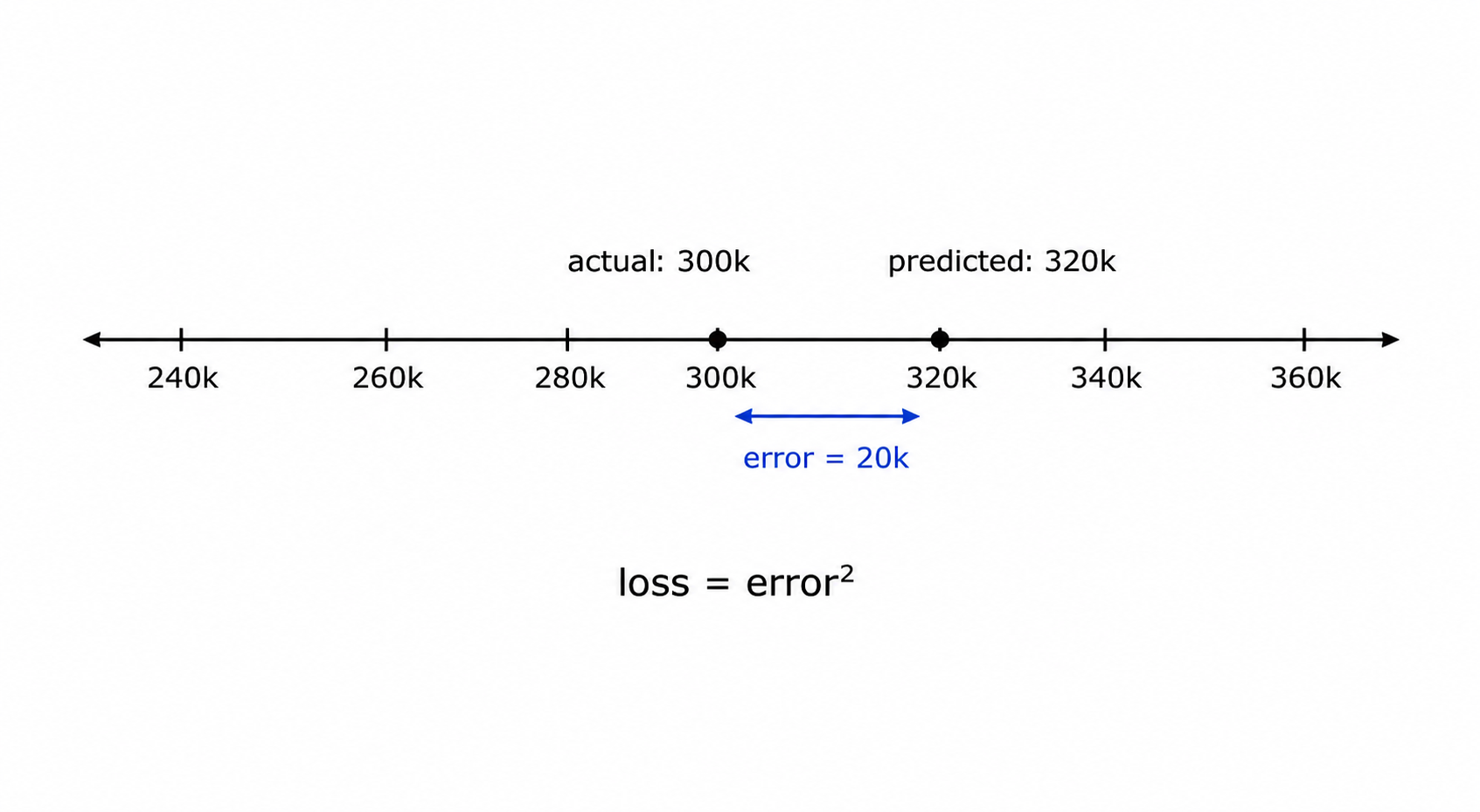
Imagine you’re training a model to predict house prices. It predicts 300,000. How wrong is that? You need one number that captures the error - something you can minimise.
That number is the loss (also called the cost or error). The lower the loss, the closer the predictions are to the correct answers. Training is the process of adjusting weights to push the loss down.
The loss function is the formula that computes this number. Different tasks need different formulas - predicting a continuous number (price, temperature) needs a different formula than predicting a category (spam/not-spam, cat/dog).
How it works
MSE - for regression
MSE (Mean Squared Error): MSE = (1/n) × Σ (predicted - actual)²
For each prediction, compute the difference from the actual value, square it, then average across all examples. Squaring does two things: it makes all errors positive (so over- and under-predictions don’t cancel), and it punishes large errors more than small ones - a 10k error, it’s 100× worse in the loss.
Pro: Smooth and differentiable everywhere - the gradient always exists, which is essential for backpropagation (post 1.4). Heavily penalises large outlier errors, so the model is pushed hard to fix its worst predictions.
Con: That same heavy penalty on outliers can be a problem if your data has genuine outliers you don’t care about - a single extreme value can dominate the loss and pull training in the wrong direction.
MAE - a simpler alternative
MAE (Mean Absolute Error): MAE = (1/n) × Σ |predicted - actual|
Instead of squaring the error, take the absolute value. A 10k error - no amplification.
Pro: More robust to outliers than MSE. Each error contributes proportionally, so extreme values don’t dominate training.
Con: Not differentiable at zero. When predicted = actual, the gradient of |x| is undefined - there’s a sharp corner. In practice this is handled with a subgradient, but it makes training less stable than MSE, especially near the minimum.
This is a preview of why differentiability matters - gradient descent (post 1.4) needs a smooth, well-defined gradient at every point to work reliably.
Huber loss - best of both
Huber loss combines MSE and MAE: it behaves like MSE for small errors (smooth, stable gradient) and like MAE for large errors (less sensitive to outliers).
Huber(δ) = 0.5 × error² if |error| ≤ δ, else δ × (|error| - 0.5 × δ)
The threshold δ controls where the switch happens. A common default is δ = 1.
Pro: Gets the stability of MSE near zero and the outlier robustness of MAE. Often a better default than either for regression tasks.
Con: One extra hyperparameter (δ) to tune. In practice the default works well enough that this is rarely an issue.
Cross-entropy - for classification
Cross-entropy loss is used when you’re predicting a category.
Before computing the loss, the network outputs a score for each class. A softmax function converts those scores into probabilities that sum to 1. Cross-entropy then measures how far that predicted probability distribution is from the true one (where the correct class has probability 1 and everything else has 0).
Cross-entropy = -log(predicted probability of the correct class)
The key insight is the -log. If the model assigns 0.9 probability to the right class, loss = -log(0.9) ≈ 0.1 - low, good. If it assigns 0.01 probability, loss = -log(0.01) ≈ 4.6 - very high. The log heavily penalises confident wrong answers.
Think of it like a confidence penalty: being unsure costs you a little, being confidently wrong costs you a lot.
Binary cross-entropy is the two-class version (spam/not-spam). Categorical cross-entropy handles more than two classes (cat/dog/bird).
Pro: Directly optimises for confident correct predictions. Differentiable everywhere (no sharp corners). Works naturally with softmax outputs.
Con: Sensitive to class imbalance - if 99% of your data is one class, the model can get low loss by always predicting that class while being useless on the rare class. Needs techniques like class weighting to handle this.
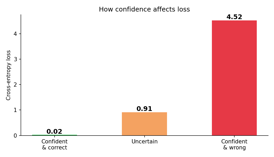
The plot below shows the loss for three scenarios - confident and correct, uncertain, and confident and wrong:
Summary
| Loss | Task | Formula | Pro | Con |
|---|---|---|---|---|
| MSE | Regression | mean((ŷ - y)²) | Smooth gradient, penalises large errors | Sensitive to outliers |
| MAE | Regression | mean(|ŷ - y|) | Robust to outliers | Not differentiable at zero |
| Huber | Regression | MSE near 0, MAE far from 0 | Best of MSE + MAE | Extra hyperparameter δ |
| Cross-entropy | Classification (multi-class) | -log(p_correct) | Optimises confidence, smooth | Sensitive to class imbalance |
| Binary cross-entropy | Classification (2 classes) | -log(p) - log(1-p) | Same as above, simpler | Same as above |
Why the choice of loss function matters
The loss function is the signal the network learns from. If you pick the wrong one, the network optimises for the wrong thing.
A concrete example: if you use MSE for a classification task, the network learns to minimise the numeric difference between its output scores and the labels (0 or 1). This works, but it doesn’t directly optimise for getting the right class with high confidence. Cross-entropy is specifically designed for that, which is why it trains faster and more reliably on classification tasks.
Getting the architecture right but the loss wrong is a common mistake. The model trains, the loss goes down, and it still performs poorly because it was optimising the wrong objective.
Code
Step 1 - MSE, MAE, and Huber on the same data:
import torch
import torch.nn as nn

predicted = torch.tensor([2.5, 0.0, 2.0, 8.0])
actual    = torch.tensor([3.0, -0.5, 2.0, 7.0])

mse_fn   = nn.MSELoss()
mae_fn   = nn.L1Loss()
huber_fn = nn.HuberLoss(delta=1.0)

print("MSE:  ", mse_fn(predicted, actual).item())
print("MAE:  ", mae_fn(predicted, actual).item())
print("Huber:", huber_fn(predicted, actual).item())
MSE: 0.1875
MAE: 0.375
Huber: 0.125Now add an outlier and watch MSE blow up while MAE stays stable:
predicted_with_outlier = torch.tensor([2.5, 0.0, 2.0, 50.0])  # last value is way off

print("MSE:  ", mse_fn(predicted_with_outlier, actual).item())
print("MAE:  ", mae_fn(predicted_with_outlier, actual).item())
print("Huber:", huber_fn(predicted_with_outlier, actual).item())
MSE: 395.1875
MAE: 10.875
Huber: 42.625One extreme prediction pushed MSE from 0.19 to 395. MAE moved from 0.38 to 10.9 - bad, but not catastrophic. Huber sits in between.
Step 2 - cross-entropy by hand on a 3-class example:
import torch
import torch.nn.functional as F

# raw scores (logits) from the network for 3 classes
logits = torch.tensor([[2.0, 1.0, 0.1]])
# correct class is 0
target = torch.tensor([0])

# by hand: softmax then -log of correct class probability
probs     = F.softmax(logits, dim=1)
loss_manual = -torch.log(probs[0, target[0]])
print("Probabilities:", probs.round(decimals=3))
print("Manual cross-entropy:", loss_manual.item())

# with PyTorch (takes raw logits, applies softmax internally)
ce_fn = nn.CrossEntropyLoss()
print("PyTorch cross-entropy:", ce_fn(logits, target).item())
Probabilities: tensor([[0.659, 0.242, 0.099]])
Manual cross-entropy: 0.417
PyTorch cross-entropy: 0.417The model assigned 65.9% probability to the correct class - not confident, but right. Loss is 0.417.
Step 3 - show how loss changes with confidence:
import matplotlib.pyplot as plt
import torch
import torch.nn.functional as F

scenarios = {
    "Confident\n& correct":  torch.tensor([[5.0, 0.5, 0.5]]),
    "Uncertain":              torch.tensor([[1.2, 1.0, 0.8]]),
    "Confident\n& wrong":    torch.tensor([[0.5, 0.5, 5.0]]),
}
target = torch.tensor([0])  # correct class is always 0
ce_fn  = nn.CrossEntropyLoss()

labels = list(scenarios.keys())
losses = [ce_fn(logits, target).item() for logits in scenarios.values()]

plt.figure(figsize=(7, 4))
bars = plt.bar(labels, losses, color=["#2dc653", "#f4a261", "#e63946"], width=0.5)
plt.ylabel("Cross-entropy loss")
plt.title("How confidence affects loss")
for bar, val in zip(bars, losses):
    plt.text(bar.get_x() + bar.get_width() / 2, bar.get_height() + 0.05,
             f"{val:.2f}", ha="center", fontsize=11, fontweight="bold")
plt.tight_layout()
plt.savefig("assets/images/1.3/cross-entropy-scenarios.png", dpi=150)
plt.show()
Confident & correct : 0.04
Uncertain : 1.10
Confident & wrong : 4.56Being confidently wrong is not just a little bad - it’s ~100× worse than being confidently right.
Key takeaways
- The loss function measures how wrong the model’s predictions are - one number per batch that training tries to minimise
- For regression: MSE is the default, MAE is more robust to outliers, Huber combines both
- For classification: cross-entropy (multi-class) or binary cross-entropy (two classes) - both heavily penalise confident wrong answers via
-log - The loss function must be differentiable everywhere for gradient descent to work - MAE’s sharp corner at zero is why MSE is usually preferred despite its outlier sensitivity
What to read next
Now we can measure how wrong the network is. The next question is: how do we use that measurement to actually fix the weights? That’s the job of gradient descent and backpropagation.