You’re in a system design interview. The interviewer says: “We’re pretraining a 70B parameter model on 2,048 GPUs. Walk me through how you’d distribute the model and where the memory goes.” If your answer stops at “we’d use DDP,” you’ve just told them you’ve never had to actually fit a model like this in GPU memory. Training a huge LLM is not “run model.fit on a bigger GPU” — no single GPU has enough memory or compute to hold the full training workload, and a real training system stitches together half a dozen techniques to get around that.
This post builds the mental model for all of them: data parallelism (DDP), tensor parallelism, pipeline parallelism, sequence parallelism, ZeRO/FSDP, activation recomputation, mixed precision, and the optimizer and learning-rate choices that make the whole thing converge.
Why Training Huge LLMs Needs More Than One GPU
A transformer needs GPU memory for five things during training: the parameters, the gradients, the optimizer states, the activations from the forward pass, and temporary communication buffers. For a small model this is a non-issue. For a huge LLM it becomes the whole problem.
Take a 7B parameter model trained in mixed precision. The FP16 weights alone are about 14 GB. Gradients in FP16 add another 14 GB. Then comes the optimizer: AdamW keeps a running momentum and variance estimate for every parameter, each stored in FP32 for numerical stability. That’s two extra FP32 copies of the model — on top of an FP32 master copy of the weights that mixed-precision training also keeps around (more on why in the mixed precision section below). Counted in “model-size units,” you’re storing roughly three full copies of the model — one for the parameters, one for momentum, one for variance — before you’ve added a single activation. Activations then scale with batch size, sequence length, and depth, and can dwarf all of the above for long-context training.
So the memory cost of training is a multiple of the model size, not the model size itself. That’s why we need multiple GPUs — and why there isn’t one way to use them. Each strategy below solves a different piece of the memory/compute/communication puzzle.
Data Parallelism: DDP
The simplest multi-GPU strategy is data parallelism — put a full copy of the model on every GPU, give each GPU a different slice of the batch, and average gradients after the backward pass. With 4 GPUs, GPU 0 gets batch A, GPU 1 gets batch B, and so on; each computes its own forward pass, loss, and gradients independently, and only synchronizes at the end of the step. After that synchronization every GPU holds the same averaged gradient and applies the same optimizer update, so all four copies stay bit-for-bit identical.
DDP: DistributedDataParallel
PyTorch’s implementation of this idea is DDP — DistributedDataParallel. One process runs per GPU, each owning a full model copy. Rank 0 broadcasts the initial weights so every process starts identical, then each GPU computes gradients on its own mini-batch, DDP averages those gradients across all GPUs, and every GPU applies the same update.
A useful analogy: four students each solve a different set of practice problems, compare their corrections, average the corrections, and every student updates their own notes using that one averaged correction. The student is the GPU, the practice problems are the local batch, the correction is the gradient, averaging the corrections is the AllReduce operation, and the notes are the model weights.
Gradient Bucketing
A neural network has hundreds of thousands of parameters. If DDP sent every parameter’s gradient as a separate message, you’d get a flood of tiny communication operations, which is slow — fewer large transfers beat many small ones on real interconnects. So DDP groups gradients into buckets — fixed-size containers that hold the gradients for many parameters — and communicates whole buckets instead of individual tensors.
Every GPU has its own local buckets; a bucket is not shared memory. Each GPU’s bucket for a given parameter group has the same layout, so before synchronization GPU 0’s bucket holds gradients computed from batch A, GPU 1’s holds gradients from batch B, and so on. After synchronization, every GPU’s bucket holds the same averaged gradient. The bucket is local; the synchronization is collective.
AllReduce: How DDP Averages Gradients
The core communication primitive in DDP is AllReduce — combine a value across every GPU and hand the combined result back to every GPU. For gradients, “combine” means sum or average. If four GPUs hold gradients 2, 4, 6, and 8, the sum is 20 and the average is 5; after AllReduce every GPU holds 5. No single GPU does all the work — every GPU participates in the collective operation. Two other collectives show up constantly in the rest of this post: AllGather, where every GPU ends up with the full concatenation of a value that was originally split across GPUs, and ReduceScatter, which combines values across GPUs but then hands each GPU only its own shard of the result instead of the full thing.
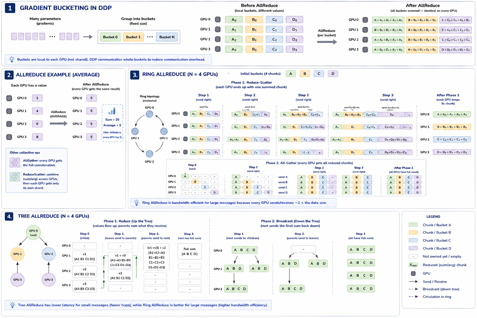 Top left: gradients are grouped into fixed-size buckets before communication. Top right: an AllReduce example averaging one value per GPU. Bottom: the same 4-GPU AllReduce worked out step-by-step for both the ring and tree algorithms.
Libraries like NCCL — NVIDIA’s Collective Communications Library, the software that actually implements these collectives efficiently on NVIDIA GPUs — offer several AllReduce algorithms. The two worth knowing are ring and tree.
Ring AllReduce. GPUs are arranged in a ring, each gradient bucket is split into chunks, and the operation has two phases:
GPU 0 → GPU 1 → GPU 2 → GPU 3 → GPU 0In the reduce-scatter phase, chunks are passed around the ring and summed as they go, so that each GPU ends up owning one fully-reduced chunk (GPU 0 has the final version of chunk A, GPU 1 has chunk B, and so on) — the result exists, but it’s scattered. In the all-gather phase, every GPU broadcasts its finished chunk to every other GPU, so each GPU ends up with the complete, fully-reduced bucket. Ring AllReduce is bandwidth-efficient for large messages because every GPU sends and receives roughly the same amount of data.
Tree AllReduce. GPUs are arranged in a tree instead of a ring. In the reduce phase, values flow upward — leaves send their gradients to their parent, the parent adds them in, and the accumulated sum climbs to the root. In the broadcast phase, the root sends the final sum back down the tree to every node. Tree AllReduce tends to win on latency for small messages, since fewer hops are needed to reach every node, while ring AllReduce tends to win on bandwidth for large messages.
The Limitation of DDP
DDP is simple and fast, but every GPU stores the full model, full gradients, and full optimizer states — none of that is sharded. If the model (plus its optimizer state) doesn’t fit on a single GPU, DDP alone can’t help you; you need a strategy that splits the model itself, not just the data.
Interview angle “Why not just use DDP for everything?” The interviewer is testing whether you understand that DDP scales compute (more data processed per step) but does nothing for memory — every GPU still needs to hold a full copy of parameters, gradients, and optimizer states. The moment the model or its optimizer state exceeds single-GPU memory, you need tensor parallelism, pipeline parallelism, or state sharding (ZeRO/FSDP), and usually some combination of all three.
Tensor Parallelism: Splitting a Layer Across GPUs
In data parallelism every GPU owns the full model. Tensor parallelism instead splits the computation inside a single layer across GPUs — useful when one layer’s matrix multiplication is too large or too expensive to run on one device. The core idea: split one huge matrix multiplication across multiple GPUs.
Tensor Parallelism in the Transformer MLP
A transformer MLP is two linear layers with a nonlinearity between them: Y = GeLU(XA), Z = YB, where X is the input activation, A and B are the two weight matrices, and Z is the output. If A is huge, split it by columns into A1 and A2. GPU 0 computes Y1 = GeLU(XA1) and GPU 1 computes Y2 = GeLU(XA2); together, Y = [Y1, Y2]. This first linear layer needs no communication, because each GPU simply owns a slice of the output. For the second matrix B, each GPU computes a partial contribution to the final output — GPU 0 produces partial Z0, GPU 1 produces partial Z1 — and the true output is Z = Z0 + Z1, which requires an AllReduce to combine. The pattern to remember: the first linear layer splits the output with no immediate communication; the second linear layer produces partial sums that need an AllReduce.
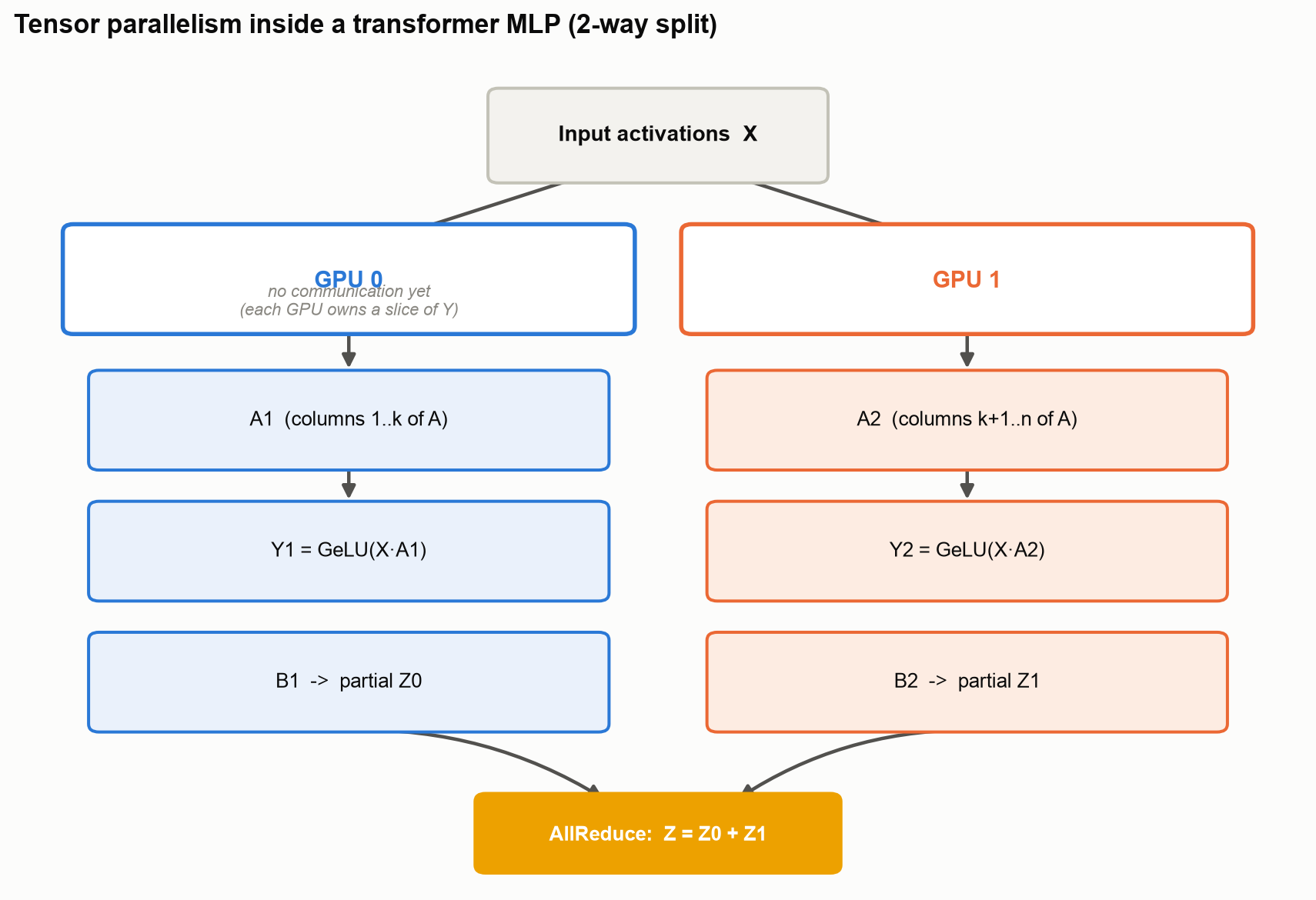 GPU 0 and GPU 1 each hold half of
 A and B. The first matmul needs no communication; the second needs an AllReduce to sum the partial outputs into Z.
Tensor Parallelism in Attention
Attention projects the input into queries, keys, and values (Q = XWq, K = XWk, V = XWv), and multi-head attention naturally has many independent heads. Tensor parallelism splits the heads across GPUs — GPU 0 handles heads 1–4, GPU 1 handles heads 5–8 — and each GPU computes attention only for its own heads. The outputs are combined through the output projection afterward, which again requires communication. Attention heads and MLP hidden dimensions are both divisible, which is exactly why tensor parallelism works cleanly on both halves of a transformer block.
Interview angle “Why is tensor parallelism usually limited to 8 GPUs, or kept within a single node?” Tensor parallelism runs an AllReduce inside every layer’s forward and backward pass — for a 40-layer model that’s 80+ collective operations per training step, each one blocking until every GPU finishes. That communication has to be fast and low-latency, which means it needs to stay on NVLink — the high-bandwidth, direct GPU-to-GPU interconnect within a node — rather than crossing to another machine over a slower network. This is why tensor-parallel degree is usually capped at the number of GPUs per node (commonly 8).
Pipeline Parallelism: Splitting Layers Across GPUs
If the full model has too many layers to fit on one GPU, split it vertically by layer: GPU 0 gets layers 1–10, GPU 1 gets layers 11–20, GPU 2 gets layers 21–30, GPU 3 gets layers 31–40. Data flows through the GPUs like an assembly line — input → GPU 0 → GPU 1 → GPU 2 → GPU 3 → output — the same way a sandwich assembly line has one worker add bread, the next add cheese, the next add vegetables, and the last wrap it.
Tensor Parallelism vs. Pipeline Parallelism
It’s worth distinguishing these two now that both are on the table, because interviewers conflate them constantly. Pipeline parallelism splits the model by layers — GPU 0 might own layers 1–10, GPU 1 layers 11–20, and so on. Tensor parallelism splits the math inside one layer — GPU 0 computes part of layer 17’s matrix multiplication while GPU 1 computes another part of the same layer, at the same time.
The Pipeline Bubble Problem
Push a single batch through that pipeline and most GPUs sit idle most of the time: while GPU 0 works in time step 1, GPUs 1–3 are idle; while GPU 1 works in step 2, GPUs 0, 2, and 3 are idle. That idle time is the pipeline bubble, and it’s the central problem every pipeline-parallelism technique below is trying to shrink.
Micro-Batches and GPipe
The fix is to split the global batch into smaller micro-batches and stream them through the pipeline back-to-back, so GPU 0 can start on micro-batch 2 the moment it hands micro-batch 1 off to GPU 1. With a 64-example batch split into four 16-example micro-batches, by time step 4 all four GPUs are simultaneously busy — GPU 0 on micro-batch 4, GPU 1 on micro-batch 3, GPU 2 on micro-batch 2, GPU 3 on micro-batch 1:
Time 1: GPU0=MB1
Time 2: GPU0=MB2  GPU1=MB1
Time 3: GPU0=MB3  GPU1=MB2  GPU2=MB1
Time 4: GPU0=MB4  GPU1=MB3  GPU2=MB2  GPU3=MB1
This exact schedule — run every micro-batch’s forward pass to fill the pipeline, then run every micro-batch’s backward pass to drain it — is what GPipe does. Forward moves left to right (GPU 0 → GPU 1 → GPU 2 → GPU 3); backward moves right to left, with each GPU computing gradients only for the layers it owns. GPipe is fully synchronous: every micro-batch in a batch uses the same weight version for both its forward and backward pass, so there’s no correctness subtlety to worry about. The cost is that the pipeline still has bubbles at the very start (filling) and very end (draining) of every batch.
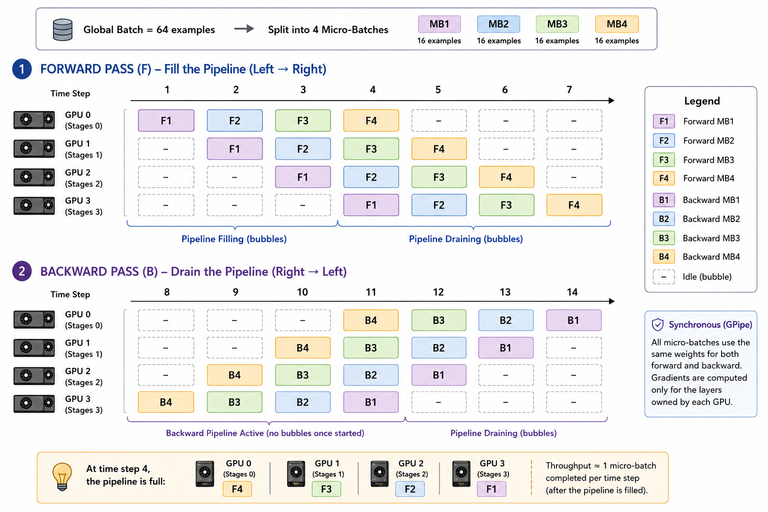 The forward wave (steps 1–7) fills then drains the pipeline; the backward wave (steps 8–14) does the same in reverse. Every micro-batch uses the same weights for both passes — the bubbles are the idle cells at each end.
PipeDream and the 1F1B Schedule
GPipe’s synchronicity is also its limitation — it never mixes forward and backward work, so the pipeline has to fully drain before a new batch starts. PipeDream takes the opposite bet: interleave forward and backward work continuously, so a GPU is never sitting idle waiting for an entire wave of forwards to finish.
PipeDream’s schedule is called 1F1B — one forward, one backward, one forward, one backward, repeating continuously — but that name undersells the actual rule, which is a cap on how far a stage is allowed to get ahead of itself. Stage s may have at most (p - s) micro-batches in flight at once — forwarded, but not yet backwarded — where p is the number of pipeline stages. That single rule produces three phases:
- Warmup. Starting from zero in-flight micro-batches, stage
sdoes forward passes until it hits its cap of(p - s), then it must wait for a backward before forwarding again. The first stage (s = 0) has the largest cap,p, so it gets to forward the furthest ahead before being forced to wait. The last stage (s = p - 1) has a cap of just1— it produces the loss itself, so it alternates forward/backward from its very first task, with no lead at all. - Steady state. Once a stage is at its cap, it does one backward (freeing up a slot) then one forward (refilling it) — the actual “1F1B” rhythm — holding a constant
(p - s)micro-batches in flight. - Cooldown. Once all
mforwards have been issued, only backwards are left; the stage drains whatever’s still in flight, mirroring the warmup count.
Here’s the verified schedule this produces for 4 stages and 8 micro-batches, forward and backward each taking one time unit (F4 = forward micro-batch 4, B1 = backward micro-batch 1, . = idle):
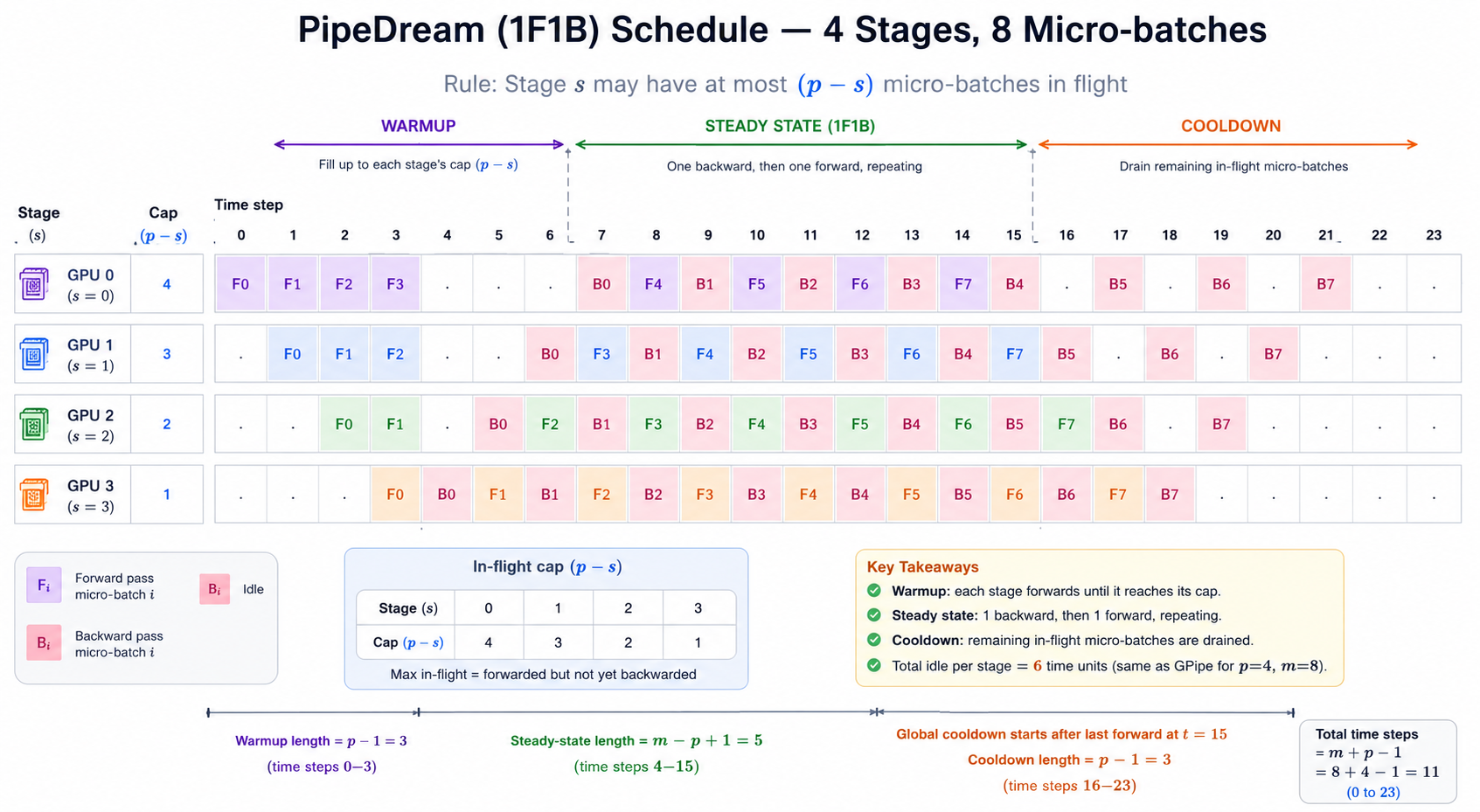 Each stage’s in-flight cap is
 (p - s), shown in the table at bottom left. Total idle per stage is 6 time units — identical to what GPipe would need for this p and m, as the “Key Takeaways” box notes.
Notice this schedule still has idle gaps — a few while each stage waits for its first backward to arrive, a matching few while it drains the last of its in-flight micro-batches — and the total idle per stage (6 units here) is exactly the same as GPipe’s would be for this p and m. Redistributing the bubble into small gaps instead of two big blocks doesn’t, by itself, remove any idle time within one batch; the “GPipe vs. PipeDream” section below covers where the real reduction comes from.
This scheduling rule is also PipeDream’s original motivating idea: the paper reports up to 5.3× faster time-to-target-accuracy than data-parallel training on image classification, and up to 4.3× on language modeling — gains that come from never pausing to fully synchronize the way GPipe does, covered next.
GPipe vs. PipeDream
Here’s the nuance interviewers actually probe: the synchronous version of 1F1B scheduling — PipeDream-Flush, covered next — does not reduce the bubble below GPipe’s. Run the schedule above for one batch and it has the exact same total idle time as GPipe would for the same p and m — 1F1B just spreads that idle time into small gaps instead of two big blocks. What it changes is memory, not idle time: GPipe must hold activations for every in-flight micro-batch until the drain phase starts (up to m micro-batches worth), while PipeDream-Flush starts a micro-batch’s backward pass the moment the last stage finishes its forward, so at most p micro-batches’ activations are ever in flight at once.
The bubble itself only shrinks when you stop paying the fill/drain cost every batch. GPipe and PipeDream-Flush both insert a full flush between batches — drain everything, apply the optimizer step, then refill from empty — so that fixed idle cost repeats every single batch. The original, fully asynchronous PipeDream never flushes: it keeps the pipeline continuously fed across batch boundaries (weight stashing is precisely what makes that safe), so the fill/drain cost is paid once at the start of training rather than once per batch. Over many consecutive batches, that’s the entire difference — same per-batch schedule, but one pays the startup cost repeatedly and the other doesn’t.
Interview angle “Does PipeDream-Flush (1F1B) actually reduce the pipeline bubble compared to GPipe?” No — this is a common misconception. Within a single batch, PipeDream-Flush has the identical idle time as GPipe; the interviewer is checking whether you know its real win is peak activation memory (only
pmicro-batches in flight instead ofm), not idle time. The bubble itself only shrinks when a schedule avoids flushing between batches — that’s what the fully asynchronous original PipeDream buys with weight stashing, and what interleaved virtual stages buy independently, covered further down.
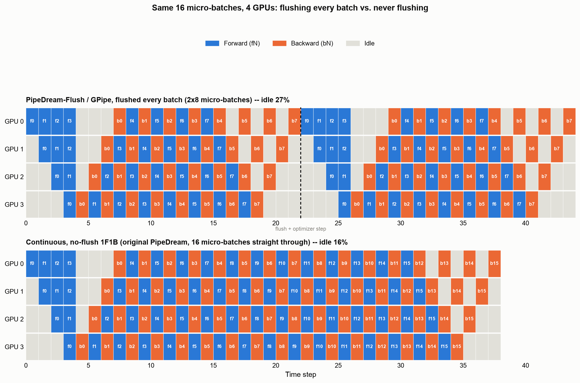 Same 16 micro-batches, same 4 GPUs, equal forward/backward time. Each cell is labeled with its micro-batch (
f3 = forward of micro-batch 3, b3 = its backward). Flushing every batch (top: two 8-micro-batch batches back to back, micro-batch numbering restarts at each flush) pays the fill/drain cost twice. Running the identical 1F1B schedule continuously with no flush (bottom, micro-batches numbered 0–15 straight through) pays it once, cutting total idle time from 27% to 16%.
Weight Stashing: Fixing PipeDream’s Stale Gradients
Running forward and backward continuously, without ever pausing for a clean batch boundary, creates a correctness problem GPipe never has: stale weights. Look at GPU 0’s sequence above — it runs F3 (a forward pass) before B1 and B2 even fire. If the optimizer applies an update after B0, then F3 and every later forward runs against newer weights than the micro-batches still waiting on their backward pass. Worse, a micro-batch’s own forward and backward can end up using two different weight versions if updates land in between — which breaks the basic assumption that a gradient is computed against the same weights it’s about to update.
The original PipeDream paper fixes this with weight stashing: each stage saves the exact weight version a micro-batch used during its forward pass, and reuses that saved version — not whatever the live weights happen to be — when that micro-batch’s backward pass runs. Correctness is restored: every micro-batch’s forward and backward see one consistent weight snapshot, even though the live weights have moved on in the meantime.
The cost is memory. Because 1F1B caps the number of micro-batches any stage keeps in flight at (p - s) — at most p, for the first stage — a stage never needs to stash more than p weight versions at once. That’s bounded and known in advance, but it’s still up to p extra copies of that stage’s weights sitting in memory beyond the single copy GPipe needs — the exact tradeoff PipeDream-2BW (below) exists to shrink.
Interview angle “How does PipeDream keep forward and backward passes correct if it never stops to synchronize?” Weight stashing: each micro-batch’s backward pass is replayed against the specific weight version its forward pass used, saved off at forward time, not against whatever the live weights are by the time backward runs. The cost is bounded by the pipeline depth
p, since that’s the max number of micro-batches 1F1B ever keeps in flight at once.
PipeDream-Flush
PipeDream-Flush keeps the 1F1B ordering (start a micro-batch’s backward as soon as possible rather than waiting for a full drain) but sidesteps stale weights the synchronous way: it stops injecting new micro-batches at the end of each global batch, lets everything already in flight finish forward and backward, updates the weights, and only then starts the next batch. That “flush” gives clean synchronous semantics — every micro-batch in a batch uses the same weight version, and the optimizer update happens only after the whole batch drains — and, as the box above lays out, leaves the bubble exactly the size GPipe’s is. What it buys instead is the memory reduction: activations for only p in-flight micro-batches instead of m.
PipeDream-2BW: Double-Buffered Weights
Flush gets memory down to p in-flight activations, but it still pays a full fill/drain bubble at every batch boundary. The original, fully asynchronous PipeDream avoids that bubble entirely by never flushing — but weight stashing then needs up to p weight versions in memory, because a micro-batch’s backward can lag its forward by as many as p - 1 steps. PipeDream-2BW (“two-buffered weights”) is the paper’s answer to getting both: no flush, and only ever 2 weight versions, regardless of how deep the pipeline is.
The trick is to stop updating the weights after every single micro-batch and instead update once per group of m micro-batches, where m is chosen to be at least the pipeline depth p (the paper’s simplifying default is m = p). Concretely, with p = 4 and groups of 4:
- Micro-batches 0–3 (group 0) use weight version
v0for both their forward and backward passes. Once every micro-batch in that group has finished its backward pass, group 0’s accumulated gradient producesv1— a new version now sitting ready for future use. - Micro-batches 4–7 (group 1) don’t get to use that new version — they were already admitted on
v0before it existed, and 2BW keeps a micro-batch on the same version for its whole forward+backward pair. So group 1 rides outv0too, and its own gradient will later producev2. - Micro-batches 8–11 (group 2) are the first to actually forward against
v1. By the time they’re ready to start, group 0 finished its backward long ago — the pipeline’s own depth-driven latency (group 1 has to fully pass through the pipeline first) already provides enough of a gap — sov1is sitting ready with no extra wait.v0isn’t discardable yet, though: it’s still being used by group 1’s still-draining backward passes. Only once micro-batch 7 (group 1’s last) finishes backward doesv0finally get freed. Right up until that moment,v0(draining) andv1(active for new forwards) are both alive at once — that overlap is the “2” in 2BW.
The net effect is a one-version-delayed gradient update — the paper writes it as W(t+1) = W(t) − ν·∇f(W(t−1)) instead of the usual W(t+1) = W(t) − ν·∇f(W(t)) — a small, bounded, and consistent staleness (every stage sees the same delay), rather than the original PipeDream’s staleness that can vary by up to p steps depending on how far a micro-batch happens to lag. A version produced by group g isn’t consumed until group g + 2 — skipping over group g + 1, which is still finishing out the version group g itself was using — and requiring m ≥ p is precisely what guarantees group g’s backward always finishes with room to spare before group g + 2 needs it, so no extra stall is required. Because of that gap, at most two versions are ever live at once: one still draining backward (group g + 1, on the older version), one active for new forwards (group g + 2, on the version group g just produced). That bound holds no matter how deep the pipeline is, which is exactly what makes 2BW scale better than weight-stashing’s p-version cost.
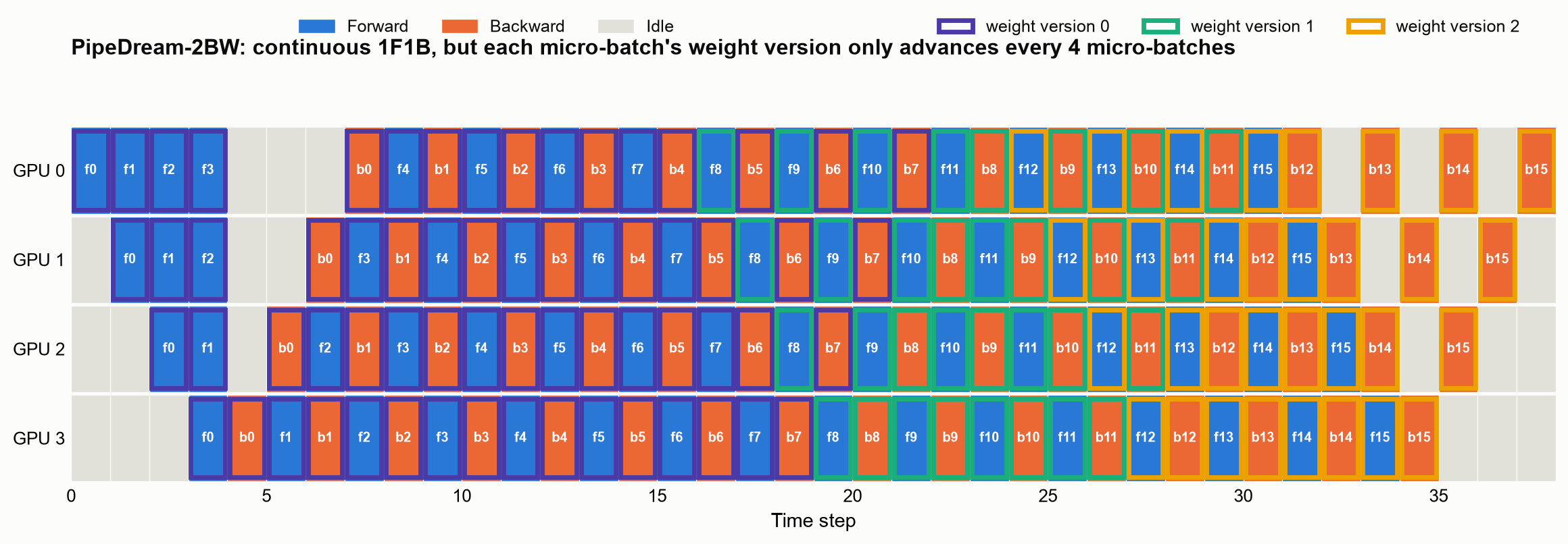 Fill color is forward/backward as before; the border color is the weight version. Version 0 (purple) covers micro-batches 0–7 — two full groups — before version 1 (green) takes over at micro-batch 8, then version 2 (gold) at micro-batch 12. At every point in this simulated schedule, at most 2 border colors are ever active across all 4 GPUs at once.
Interview angle “How does PipeDream-2BW bound memory to exactly 2 weight versions when the original PipeDream needs up to
p?” By updating weights once per group ofm ≥ pmicro-batches instead of once per micro-batch, and by having a version skip a full group before it’s consumed: the version groupgproduces isn’t used until groupg + 2, not groupg + 1. Requiringm ≥ pguarantees groupg’s backward always finishes well before groupg + 2needs its gradient, so admission never has to stall waiting for it. The two versions alive at any moment are the one still draining (groupg + 1, finishing out the older version) and the one just starting to be used (groupg + 2) — never three, because groupg + 1’s backward always finishes before groupg + 3would need yet another version. The cost is a bounded, one-version-delayed gradient update (∇f(W(t−1))instead of∇f(W(t))) — worse than Flush’s zero staleness, but far cheaper to bound than the original PipeDream’s staleness, which scales with pipeline depth.
Does the One-Version Delay Actually Hurt Convergence?
A gradient computed one version behind — ∇f(W(t−1)) instead of ∇f(W(t)) — is still a form of staleness, so it’s a fair question whether it costs anything in practice. The paper’s argument for why it doesn’t starts from a simple observation: weights move by one optimizer step’s worth between W(t−1) and W(t), and a single step is small relative to the weights themselves, so W(t) ≈ W(t−1) — the gradient computed against the slightly older version is a good-enough approximation of the gradient against the current one. Applied at the granularity of a group (m ≥ p micro-batches, not a single step), that approximation only gets better, since the delay is one group’s update, but each group’s gradient is itself already an average over m micro-batches.
The paper backs this with real convergence numbers rather than just the intuition. Fine-tuning BERT models pretrained with 2BW against a non-pipelined (“vanilla”) baseline, downstream accuracy was statistically indistinguishable: 87.82% vs. 87.77% on MNLI, 79.48% vs. 80.06% on RACE. For GPT trained on Wikitext-103, 2BW and vanilla landed at nearly identical test perplexity (19.56 vs. 19.28) — and matched exactly once the vanilla run was given 20% fewer iterations, i.e. once you account for the fact that 2BW’s lack of pipeline flushes lets it complete more iterations in the same wall-clock time. The loss curves tell the same story over training: 2BW tracks the vanilla loss curve almost exactly after the first ~100K iterations, with the small gap that exists showing up earlier in training, when the weights are changing fastest and the one-version-old gradient is the roughest approximation of the current one.
Notably, none of this required extra machinery — no learning-rate compensation, no gradient smoothing across versions, no weight prediction. The stale gradient is just fed directly into the optimizer (m_t = β·m_(t−1) + (1−β)·∇f(W(t−1)) for a momentum-based optimizer, with no correction term). The one caveat the authors do flag: for models that only support very small batch sizes, 2BW, PipeDream-Flush, and GPipe all become less attractive, since all three do their gradient accumulation inside the pipeline schedule itself — at small batch sizes there isn’t enough micro-batching headroom to fill the pipeline without shrinking each micro-batch to the point of hurting hardware utilization.
Interview angle “Why is it safe for PipeDream-2BW to train on a gradient that’s one version stale?” Because weights change by only one optimizer step between consecutive versions, so
W(t) ≈ W(t−1)and the stale gradient is a close approximation of the current one — and the paper backs this empirically, not just intuitively: BERT downstream accuracy and GPT perplexity both come out statistically indistinguishable from a non-stale baseline, with no learning-rate or gradient corrections needed. The place this reasoning breaks down is very small batch sizes, where gradient accumulation has to happen inside the pipeline schedule and there isn’t enough micro-batching room to do it without hurting utilization.
Interleaved Pipeline Parallelism
A normal pipeline gives each GPU one continuous chunk of layers. Interleaved pipeline parallelism instead gives each GPU several smaller, non-contiguous chunks — GPU 0 might own layers 1–2 and layers 9–10, GPU 1 owns layers 3–4 and 11–12, and so on — so each physical GPU participates in the pipeline multiple times as a different “virtual stage.” When a GPU would otherwise be idle waiting on its next chunk in the main sequence, it can instead work on one of its other chunks. If each GPU holds v model chunks, the pipeline bubble shrinks by roughly a factor of v, at the cost of more communication and more complex scheduling.
Sequence Parallelism: Sharding the Sequence Dimension
Tensor parallelism shards the matrix multiplications inside attention and the MLP, but not every operation in a transformer block gets sharded by it — layernorm and dropout, for instance, still run on the full sequence on every tensor-parallel GPU, so their activations are duplicated t times across a t-way tensor-parallel group (using t for tensor-parallel degree, matching the memory formulas below). That duplication becomes a real memory problem at long context lengths, since activation memory scales linearly with sequence length.
Sequence parallelism closes that gap by splitting the sequence dimension of activations across the same GPUs already used for tensor parallelism, so no single GPU ever holds activations for the full sequence — just its own shard of tokens — for the operations tensor parallelism doesn’t already shard. It’s not a competing strategy to tensor parallelism; it rides along inside the same tensor-parallel group and specifically targets the activation memory that tensor parallelism leaves untouched.
Walking Through One Transformer Block
A transformer block alternates between two kinds of regions, and sequence parallelism only touches one of them. LayerNorm, dropout, and the residual adds operate independently on each token — nothing about them needs to see the full sequence at once — so they run in a sequence-parallel region: each of the t GPUs holds only its own s/t slice of the sequence, for every tensor it touches. Self-attention and the MLP, by contrast, are the tensor-parallel regions: attention needs every token to compute its heads, and the MLP’s matmuls are split by hidden dimension, not by sequence — so both need the full sequence length on every GPU, just a shard of the hidden dimension.
That means every time execution crosses from one region into the other, the activation’s shape has to change — sequence-sharded (s/t, b, h) on one side, full-sequence (s, b, h) on the other — and that reshaping is the communication:
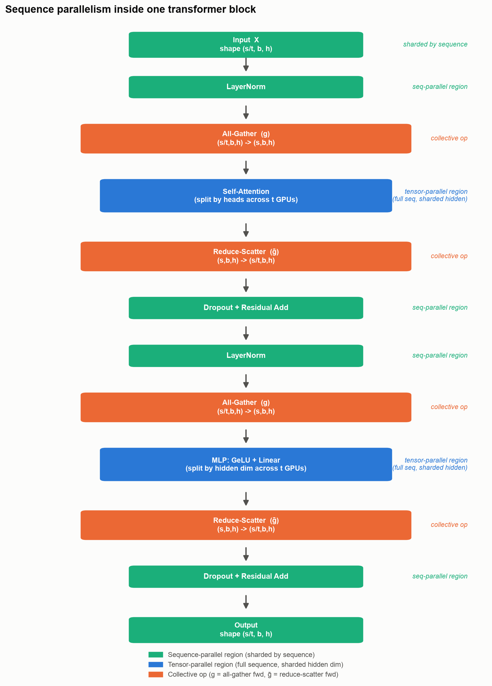
g is an all-gather in the forward pass (and becomes a reduce-scatter in the backward pass); ḡ is a reduce-scatter in the forward pass (and an all-gather in the backward pass). Every transformer block does two of each per direction — one pair around attention, one pair around the MLP.
Going into a tensor-parallel region, an all-gather reassembles the full sequence from every GPU’s shard. Coming out of one, the tensor-parallel matmul has already produced a partial sum per GPU (the same partial-sum situation plain tensor parallelism resolves with an AllReduce) — but instead of an AllReduce, sequence parallelism uses a reduce-scatter, which sums those partial results and hands each GPU back only its own sequence shard in the same step.
Why the Extra Communication Is Free
Splitting one AllReduce into an all-gather-plus-reduce-scatter sounds like it should cost more, but it doesn’t — because that’s already how ring AllReduce works internally. Back in the “AllReduce: How DDP Averages Gradients” section earlier, ring AllReduce was built from exactly two phases: reduce-scatter, then all-gather, moving the same total bytes either way. Sequence parallelism just stops after the reduce-scatter half in one spot and does the all-gather half at the next region boundary instead of immediately — same two operations, same total bytes moved, just relocated to where the sequence-sharded/full-sequence transition actually needs them. Megatron’s own framing of this: total communication volume for tensor parallelism with sequence parallelism equals plain tensor parallelism’s communication volume. You get the extra sharding of layernorm and dropout activations for zero additional bytes on the wire.
The Memory Win, Concretely
For a transformer layer with sequence length s, batch size b, hidden size h, a attention heads, and tensor-parallel degree t, plain tensor parallelism’s per-layer activation memory works out to sbh(10 + 24/t + 5as/ht) — that leading 10sbh term is exactly the replicated layernorm/dropout activations, and it doesn’t shrink no matter how large t gets. Add sequence parallelism, and the whole expression collapses to (sbh/t)(34 + 5as/h) — the entire formula, not just the already-sharded portion, now divides cleanly by t. Double the tensor-parallel degree and activation memory per GPU exactly halves, instead of asymptotically approaching a floor set by that stubborn 10sbh term.
Interview angle “You’re training with 128K context and running out of activation memory even with tensor parallelism on. What do you reach for?” Tensor parallelism shards the big matrix multiplications, but layernorm and dropout activations are still replicated across the tensor-parallel group — that’s a
10sbh-sized cost that doesn’t improve as you add more tensor-parallel GPUs. Sequence parallelism shards those along the sequence dimension inside the same group, turning the whole per-layer activation formula into something that scales down linearly with tensor-parallel degree, for no extra communication (the all-gather/reduce-scatter pair it adds is the same total bytes an AllReduce would’ve moved anyway). Combine it with activation recomputation (below) and you get the two standard levers for long-context training.
Combining Everything: 3D (PTD-P) Parallelism and Multi-Node Topology
Huge LLM training combines pipeline (P), tensor (T), and data (D) parallelism at once — often called PTD-P. Tensor parallelism splits one layer’s computation across GPUs; pipeline parallelism splits the model’s layers across groups of GPUs; data parallelism replicates the whole pipeline/tensor-parallel unit and feeds each replica different data, synchronizing gradients across replicas the same way plain DDP does.
A Worked 1024-GPU Example
A concrete layout for training a massive transformer on 1,024 GPUs:
Tensor parallel size   = 8
Pipeline parallel size = 8
Data parallel size     = 16
Total: 8 × 8 × 16 = 1024 GPUs
Tensor parallel size 8 means each transformer layer’s matrix multiplications are split across 8 GPUs. Pipeline parallel size 8 means the model’s layers are split into 8 stages — early layers on stage 0, later layers on stage 7. Data parallel size 16 means there are 16 full replicas of that tensor-and-pipeline-parallel unit, each processing different data, with gradients synchronized across all 16 replicas at the end of each step.
NVLink vs. InfiniBand: Why Topology Dictates the Parallelism Layout
The 8×8×16 split above isn’t arbitrary — it follows directly from the physical network. NVLink is the direct, high-bandwidth interconnect between GPUs inside the same server node (hundreds of GB/s, low latency); InfiniBand is the network fabric connecting different nodes to each other, with meaningfully lower bandwidth and higher latency than NVLink.
Tensor parallelism’s AllReduce fires inside every single layer’s forward and backward pass — the most communication-frequent, most latency-sensitive workload in the whole stack — so it needs to stay on NVLink, which caps tensor-parallel degree at the GPU count per node (usually 8). Pipeline parallelism only communicates activations at stage boundaries, far less frequently, so pipeline stages can span multiple nodes over InfiniBand without much penalty. Data parallelism’s gradient AllReduce happens once per step and can be overlapped with backward compute, so it also tolerates crossing nodes over InfiniBand. That’s the practical rule: tensor parallelism within a node, pipeline and data parallelism across nodes.
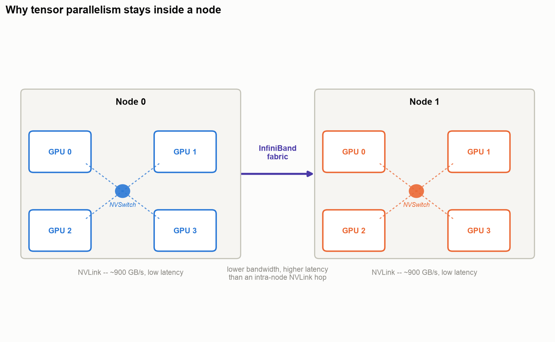 Tensor parallelism’s per-layer AllReduce has to stay inside the NVLink mesh within one node. Pipeline and data parallelism communicate far less often, so they’re the axes that cross the slower InfiniBand fabric between nodes.
Interview angle “Why is tensor-parallel size almost always 8 or less, and never crosses nodes?” Because it maps to the number of GPUs per node connected by NVLink, and tensor parallelism’s per-layer AllReduce is too latency-sensitive to survive going over InfiniBand to another machine. Pipeline and data parallelism communicate far less often and can absorb that extra latency, which is why they’re the axes you scale across nodes.
ZeRO and FSDP: Sharding Model State
DDP stores redundant state — every GPU holds full parameters, full gradients, and full optimizer states, and for AdamW that optimizer state is especially large. ZeRO and FSDP attack this directly by sharding training state across GPUs instead of replicating it.
ZeRO Stages 1, 2, 3
ZeRO — Zero Redundancy Optimizer — shards state in three increasingly aggressive stages.
Stage 1 shards only the optimizer states; parameters and gradients stay fully replicated on every GPU. Since AdamW’s optimizer states are the single largest chunk of training memory, this alone is a meaningful win: GPU 0 keeps full weights and full gradients but only optimizer shard 0, GPU 1 keeps optimizer shard 1, and so on. Crucially, because parameters are still fully replicated, forward and backward run exactly like DDP — no extra communication, no gathering — the only new step is that after the usual gradient AllReduce, each GPU applies the optimizer update using only its own shard of the (now fully-replicated-but-locally-sliced) gradient and its own optimizer-state shard, then AllGathers the tiny handful of updated weight slices back into full replication for the next step.
Stage 2 shards optimizer states and gradients, keeping only parameters replicated — GPU 0 keeps full weights but only gradient shard 0 and optimizer shard 0. Forward is still untouched (parameters are replicated, so no gathering needed). Backward changes: instead of an AllReduce that leaves every GPU with the full averaged gradient, ZeRO-2 uses a ReduceScatter, so each GPU ends up with only its own shard of the averaged gradient — the full gradient tensor is never materialized anywhere. This saves more memory than Stage 1, at the cost of that ReduceScatter replacing what used to be a plain AllReduce.
Stage 3 shards everything — parameters, gradients, and optimizer states are all split across GPUs, so GPU 0 holds only weight shard 0, gradient shard 0, and optimizer shard 0. This is the most memory-efficient stage, but now forward changes too: a layer’s forward or backward pass needs the full weight to compute against, and no GPU has that on its own anymore, so ZeRO-3 has to temporarily gather the needed shards from other GPUs before every layer’s compute, then free them again immediately after. That’s the mechanism worth walking through in detail, since it’s the one stage where sharding actually reaches into the compute path — covered next under FSDP, which implements the identical scheme.
FSDP: Fully Sharded Data Parallel
FSDP — Fully Sharded Data Parallel — is PyTorch’s implementation of the same idea as ZeRO Stage 3: each GPU stores only a shard of parameters, gradients, and optimizer states, and full parameters are gathered only when a layer actually needs them for computation. Each GPU still processes its own slice of data, exactly like data parallelism — the difference from DDP is that model state is sharded instead of fully replicated. In short: DDP is replicated data parallelism, FSDP is sharded data parallelism.
The all-gather at the heart of this happens one layer at a time, not once for the whole model. Walking through one layer end to end, on 4 GPUs, each holding a quarter of that layer’s weights (W0–W3):
- Steady state. Between layers, each GPU holds nothing but its own weight shard — no full parameter, no full gradient, no full activation. This is the memory-saving state FSDP spends as much time in as possible.
- Before forward: All-Gather. Just before this layer runs, every GPU sends its shard to every other GPU, so all 4 GPUs end up holding the full layer weight — temporarily.
- Forward compute. Every GPU now runs the exact same full layer forward pass — but on its own micro-batch of data, exactly like data parallelism. This step needs zero communication: nothing about the activations gets shared between GPUs, because activations were never the thing being sharded — only the parameters were. Each GPU produces its own local activations from the same weights applied to different data.
- After forward: discard. The moment this layer’s forward is done, each GPU throws away the full gathered copy and keeps only its own shard again. If it needed the full weight again — say, for backward — it’ll re-gather then.
- Before backward: All-Gather again. Once backward reaches this layer, the full weight gets gathered a second time (FSDP’s default is to not keep the gathered copy around between forward and backward, trading a second All-Gather for lower peak memory).
- Backward compute. Each GPU computes gradients using the full weight and its own locally-stored activations from step 3. This produces a full-sized gradient tensor on every GPU — but each one reflects only that GPU’s own micro-batch, so the four copies differ and none of them is the “real” answer yet.
- Reduce-Scatter. The four full-sized gradient tensors get summed and split in one collective operation: GPU 0 ends up with only shard 0 of the properly-averaged gradient, GPU 1 with shard 1, and so on. No GPU ever holds the full averaged gradient.
- Optimizer step: fully local. Each GPU updates its own weight shard using its own gradient shard and its own optimizer-state shard. No communication at all — everything needed for this step was already local.
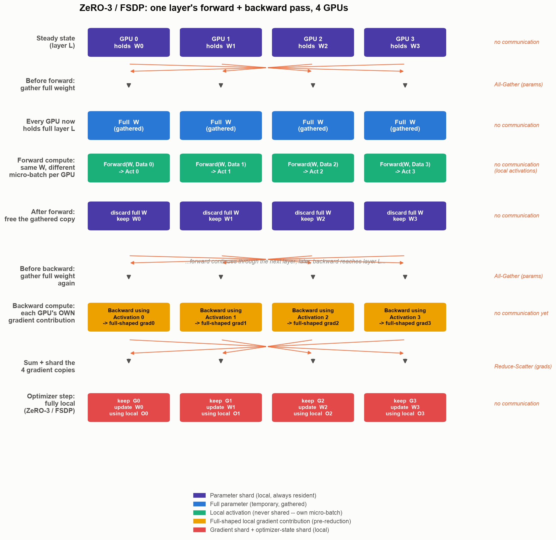 Purple = parameter shards, always resident. Blue = the full parameter, only ever temporary. Green = activations — always local, never gathered or scattered, because ZeRO/FSDP never shards them. Yellow = each GPU’s own full-shaped gradient contribution before reduction. Red = the final gradient shard and optimizer-state shard used for the fully local update.
The one thing that never gets sharded, gathered, or scattered anywhere in this picture is the activation — every GPU computes and keeps its own activations from its own micro-batch, exactly as it would under plain DDP. ZeRO and FSDP shard model state (parameters, gradients, optimizer states); the data-parallel dimension — different data per GPU, private activations per GPU — is untouched and layered on top, same as it’s always been since the very first DDP section of this post.
Why Peak Memory Isn’t the Whole Model
Steps 2–4 above repeat separately, one layer at a time — the all-gather for layer 2 doesn’t happen until layer 1’s gathered copy has already been discarded. Because every GPU moves through layers in lockstep (same order, same timing, since this is still one synchronous data-parallel forward pass), at any single instant only one layer’s full weight exists anywhere across the whole fleet — never all of them at once. That’s the entire reason the transient cost is “one layer’s worth” rather than “the whole model’s worth”: it’s not a fraction carved out of a bigger gather, it’s the same per-layer gather repeated L times, each one cleaned up before the next begins.
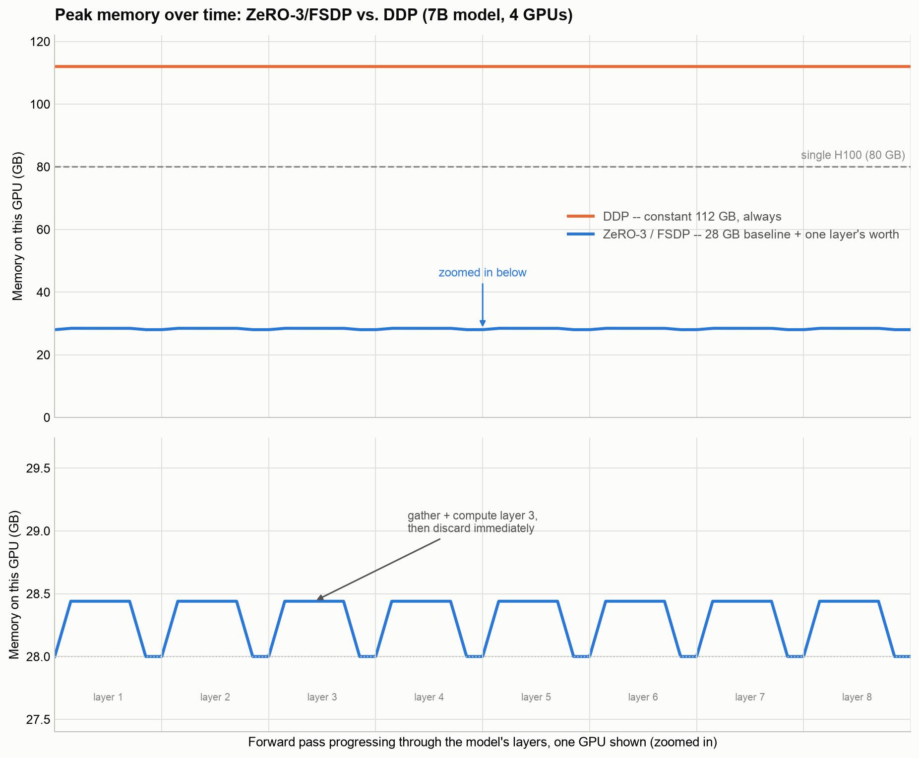 Top: DDP holds a constant 112 GB for this 7B model — more than an 80 GB GPU has. ZeRO-3/FSDP sits at a 28 GB baseline throughout. Bottom: zoomed into just the ZeRO-3/FSDP line, the sawtooth is one small bump per layer (gather → compute → discard), each returning fully to baseline before the next layer’s bump starts.
Interview angle “If ZeRO-3 has to gather the full weight before every layer’s forward pass, isn’t peak memory basically the same as DDP?” No — the gather is scoped to one layer, not the whole model, and it’s freed before the next layer’s gather even starts. Because every GPU processes layers in the same order at the same time, only one layer’s full weight is ever materialized across the entire fleet at any instant. Peak memory is the permanent shard (params + grads + optimizer states, divided by GPU count, for all layers) plus one layer’s transient full weight — for a model with dozens of layers, that transient piece is a rounding error next to the steady-state savings, not a second copy of the whole model.
DDP vs. ZeRO vs. FSDP
| Method | Parameters | Gradients | Optimizer states | Memory saving | Communication volume |
|---|---|---|---|---|---|
| DDP | replicated | replicated | replicated | low | baseline (1x) |
| ZeRO-1 | replicated | replicated | sharded | medium | same as DDP (1x) |
| ZeRO-2 | replicated | sharded | sharded | high | same as DDP (1x) |
| ZeRO-3 / FSDP | sharded | sharded | sharded | highest | up to 1.5x DDP |
The rule of thumb: more sharding buys less memory, and — contrary to what you might expect — that’s free for the first two stages. Sharding just optimizer states (ZeRO-1) or optimizer states plus gradients (ZeRO-2) doesn’t add any communication over plain DDP; it’s only ZeRO-3/FSDP’s parameter sharding that raises the communication bill. Use DDP when the model comfortably fits; reach for ZeRO-1/2 for free memory headroom; reach for FSDP/ZeRO-3 the moment the model or its optimizer state doesn’t fit even with 1 and 2’s savings.
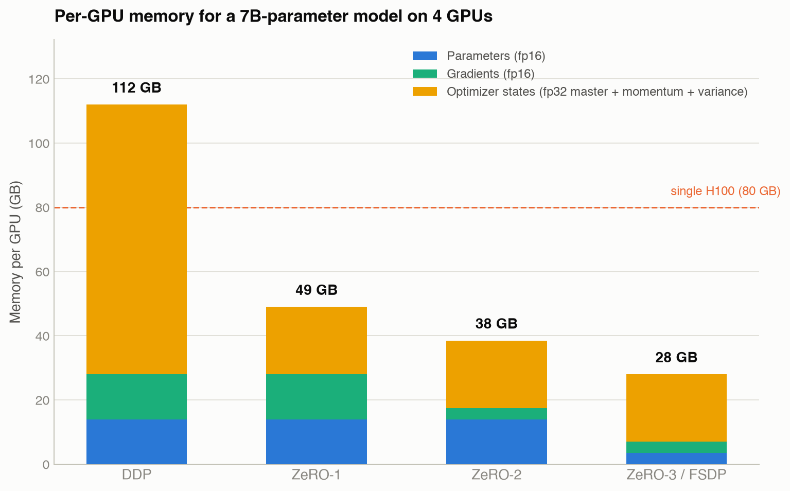 A 7B model in mixed-precision AdamW training needs about 112 GB per GPU under plain DDP — more than a single 80 GB GPU has. Progressive sharding brings that down to 28 GB under ZeRO-3/FSDP on 4 GPUs.
Interview angle “When would you pick ZeRO-2 over ZeRO-3/FSDP?” If the model’s parameters fit comfortably in memory but the optimizer states and gradients don’t, ZeRO-2 gets most of the memory win without paying for the parameter all-gather that ZeRO-3/FSDP needs on every layer. ZeRO-3/FSDP is for the case where even the parameters themselves don’t fit — the extra communication is the price of training a model that literally couldn’t exist on that hardware otherwise.
The Memory-for-Communication Trade, With Real Numbers
“More communication” is easy to say and easy to overestimate. Both the original ZeRO paper and the PyTorch FSDP paper give an actual number for it, and they agree: ZeRO-1 and ZeRO-2 add zero communication over DDP — the AllReduce just gets restructured into a reduce-scatter, same total bytes — while ZeRO-3/FSDP’s extra parameter all-gathers bring total communication volume to up to 1.5x DDP’s. That’s not symmetric with the memory savings, which is exactly the point:
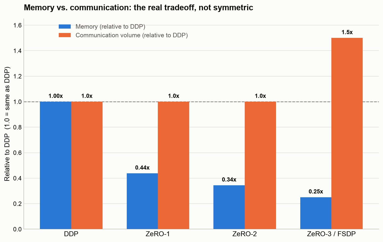 Memory drops steadily across all three stages (1.00x → 0.44x → 0.34x → 0.25x of DDP, using the same 7B/4-GPU numbers as the chart above). Communication volume stays completely flat at DDP’s level for ZeRO-1 and ZeRO-2, and only jumps — to 1.5x, not gradually — at ZeRO-3/FSDP.
1.5x more bytes moved doesn’t translate to 1.5x slower, though, for reasons both papers measured directly rather than just asserted:
- Overlap hides most of it. The FSDP paper measured an 18% speedup on a 175B model from backward prefetching alone — starting the next layer’s all-gather while the current layer’s backward is still computing, instead of doing them serially.
- The measured hit is often much smaller than 1.5x. Scaling an 11B model from 8 to 512 GPUs (64x), the same paper measured only a 7% regression in per-GPU TFLOPS — and on smaller models (611M–2.28B parameters) FSDP and DDP throughput came out “similar” despite FSDP doing full sharding the whole time.
- Freed-up memory buys bigger batches, which buys throughput back. The ZeRO paper calls this out explicitly: scaling a 60B model from 64 to 400 GPUs, measured throughput more than doubled — super-linear — because the memory ZeRO-3 frees up let them run larger batch sizes per GPU, and larger batches mean higher arithmetic intensity independent of the communication cost.
- Sometimes there’s no comparison to make at all. On an 11B model in the FSDP paper, plain DDP simply runs out of memory. The “cost” of ZeRO-3 there isn’t a slowdown relative to DDP — it’s the difference between the run happening and not happening.
Interview angle “Doesn’t ZeRO-3’s 1.5x communication mean it’s 1.5x slower than DDP?” No — that’s bytes moved, not wall-clock time. Well-engineered overlap (prefetching the next layer’s all-gather during the current layer’s backward) hides most of it; measured regressions in the FSDP paper are closer to single digits at large scale, not 50%. And the memory it frees up often buys back more throughput than the communication costs, via larger batch sizes — the original ZeRO paper measured super-linear scaling from exactly this effect.
Activation Recomputation
Parameters, gradients, optimizer states, and communication aren’t the whole memory story — LLM training also burns a lot of memory on activations, the intermediate outputs of the forward pass (x1 = layer1(x0), x2 = layer2(x1), and so on) that the backward pass needs in order to compute gradients. Naively, training saves every one of these, which is expensive at depth.
Activation recomputation — also called activation checkpointing or gradient checkpointing — trades compute for memory: instead of saving every activation, save only a handful of checkpoints, and recompute the missing ones on demand during backward. With 8 layers, instead of saving x1 through x8, save only x0, x2, x4, x6, x8; if backward needs x5, recompute it on the fly as x5 = L5(x4).
The Memory Math Behind sqrt(l) Checkpointing
Without recomputation, activation memory scales as O(l) for an l-layer model — you’re saving activations for every layer. With recomputation, split the model into d partitions; memory then has two components: the activations you need to hold inside one partition (O(l/d)) plus the checkpoints you save at partition boundaries (O(d)). Those two terms are minimized together when l/d ≈ d, i.e. d ≈ sqrt(l), which brings total activation memory down to roughly O(sqrt(l)) — a big improvement over O(l).
Concretely, for a 100-layer model, naive activation memory is proportional to 100. Checkpointing with d = sqrt(100) = 10 means storing about 10 checkpoints, with each partition needing to temporarily hold about 10 layers’ worth of activations during its local recomputation — roughly 20 total, instead of 100.
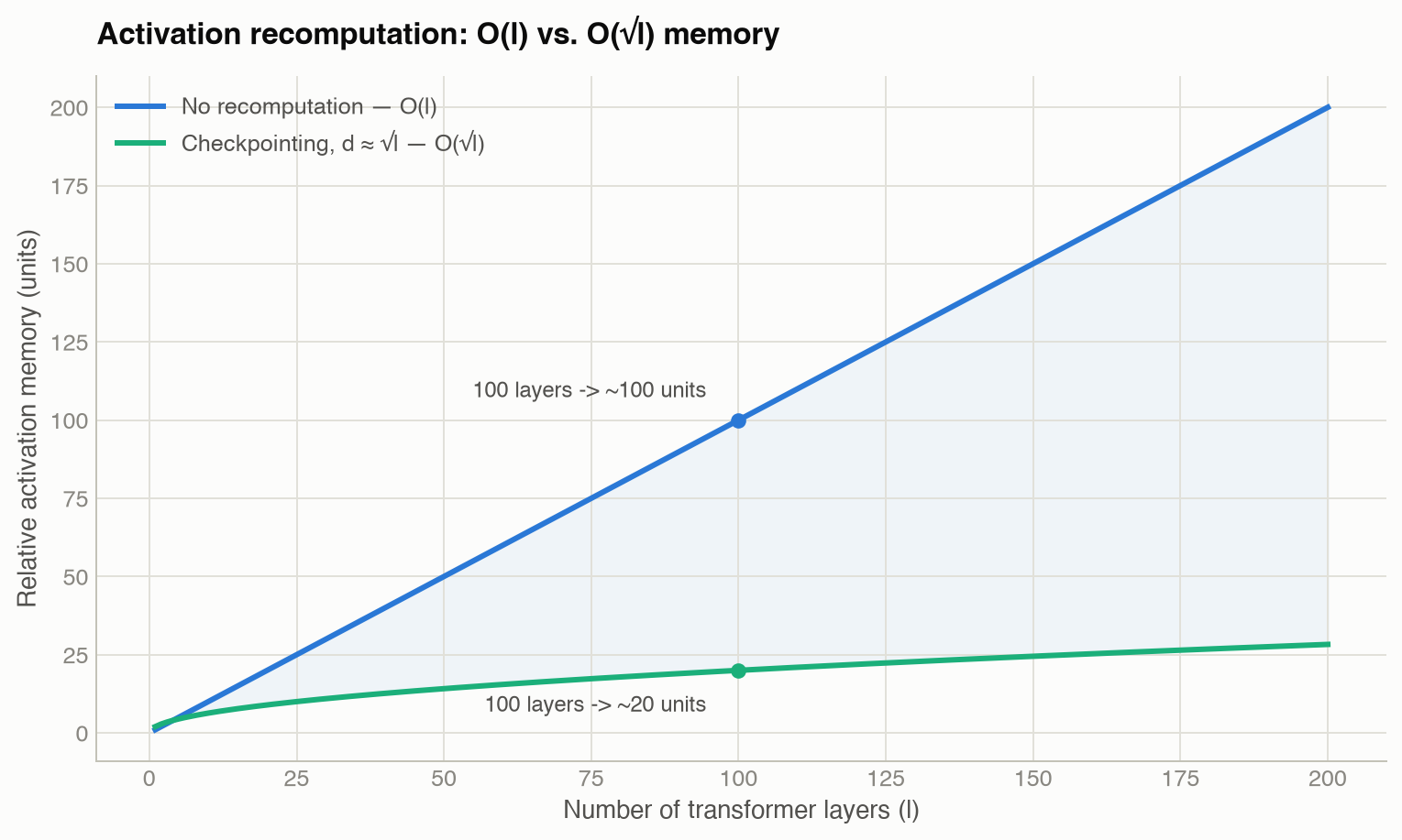 The gap between the two curves widens as models get deeper — at 100 layers, checkpointing needs roughly a fifth of the activation memory naive training does.
Selective Activation Recomputation
Checkpointing every layer boundary recomputes everything uniformly, but not every operation costs the same to recompute relative to how much activation memory it saves. Selective activation recomputation exploits this: recompute only the cheap-to-recompute, memory-heavy operations (attention is a common target — it’s relatively cheap in FLOPs but produces large intermediate tensors), while keeping the activations for the expensive-to-recompute parts (like the MLP) stored rather than recomputed. This gets most of the memory benefit of full checkpointing while paying much less of the compute penalty, because you’re only re-running the parts of the forward pass that were cheap in the first place.
Why It Matters More for Long Context
Activation memory scales with batch size × sequence length × hidden dimension × number of layers. Double the sequence length and activation memory grows in proportion — for long-context training, activations, not parameters, are often the binding constraint. Activation recomputation is what makes training with larger models, longer sequences, or larger micro-batches possible at all; the cost is that parts of the forward pass run twice.
Interview angle “Your activation memory is the bottleneck for a long-context run — walk me through your options in order.” Reach for activation recomputation first (recompute rather than store, ideally selectively so you’re not recomputing the expensive parts), then sequence parallelism (shard the activations that tensor parallelism doesn’t already shard along the sequence dimension), and only then consider shrinking batch size or micro-batch size, since that directly hurts training throughput and gradient estimate quality.
Mixed Precision Training
Mixed precision training uses lower-precision numbers for most computation while keeping sensitive state in higher precision. FP32 (32-bit floating point) is accurate but memory- and compute-heavy; FP16 and BF16 (16-bit formats) use half the memory and run faster on modern GPUs, but not without complications.
FP16 causes two concrete failure modes. Underflow: a tiny gradient like 0.00000001 is representable in FP32 but can round to exactly 0 in FP16, silently killing that learning signal. Vanishing updates: an update of 0.000001 applied to a weight of 1.0000 can round right back to 1.0000 in low precision — the update simply disappears.
FP32 Master Weights and Loss Scaling
Classic mixed precision training keeps an FP32 master copy of the weights alongside the fast FP16 working copy: cast weights to FP16 for the forward and backward pass, compute gradients, but apply the optimizer update to the FP32 master weights, then re-cast the result back to FP16 for the next step. Forward and backward stay fast; the update itself stays numerically accurate.
Loss scaling solves the underflow problem directly: multiply the loss by a large constant (say 1024) before backward, which scales every gradient in the chain by the same factor, then divide the resulting gradients back down by that same constant before applying them. This keeps small gradients above FP16’s representable range during backward without changing the final update. Some accumulations — a long dot product, for instance — are also run in higher precision internally even when inputs and outputs stay in FP16/BF16 (multiply in low precision, accumulate in FP32, store the result in low precision), which limits how much rounding error can build up across many additions.
BF16 vs. FP16
BF16 — brain floating point — trades mantissa precision for exponent range: it has less precision than FP16 but a dynamic range similar to FP32, which makes it far less prone to the overflow/underflow problems FP16 has, and often removes the need for loss scaling entirely. For most LLM training today, BF16 is preferred specifically because of this stability, not because it’s more accurate — FP16 actually has more mantissa bits when it doesn’t overflow or underflow.
FP8: Pushing Precision Further
FP8 halves the memory of BF16 again by using only 8 bits per value, at the cost of an even smaller dynamic range that FP16 or BF16. Because that range is so limited, FP8 training needs active, often per-tensor or per-block, dynamic scaling to keep values inside the representable range — it isn’t a drop-in replacement the way BF16 was for FP16. FP8 is primarily used for the matrix multiplications themselves on hardware that supports it (H100-class GPUs via NVIDIA’s Transformer Engine), while accumulation and the optimizer’s master weights stay in a higher-precision format, the same layered strategy mixed precision has always used, just pushed one level lower.
Interview angle “Why does BF16 need less babysitting than FP16?” FP16 has a narrow dynamic range, so gradients underflow to zero or updates vanish unless you actively manage it with loss scaling. BF16 keeps FP32’s exponent range (same number of exponent bits) while sacrificing mantissa precision, so it rarely under/overflows in the first place — that’s why most LLM pretraining today skips loss scaling entirely and just uses BF16.
Batch Size and Gradient Accumulation
Larger batches generally mean more stable training and better gradient estimates, but GPU memory caps how large a single forward/backward pass can be. Gradient accumulation breaks the gap: run several forward/backward passes on smaller micro-batches, summing their gradients without applying an optimizer step, then apply one optimizer update after the accumulated gradients represent the full intended batch. This simulates a large batch on limited memory at the cost of extra wall-clock time — you’re trading throughput for memory, the same trade activation recomputation makes.
The effective batch size you’re actually training with is:
effective_batch_size = per_GPU_micro_batch_size × gradient_accumulation_steps × num_data_parallel_GPUsIf each of 8 data-parallel GPUs runs a micro-batch of 4 examples and accumulates over 8 steps before updating, the effective batch size is 4 × 8 × 8 = 256, even though no single forward pass ever sees more than 4 examples at once.
Interview angle “You want a bigger effective batch size but you’re already at the GPU’s memory limit per micro-batch. What are your levers?” Gradient accumulation (more steps before the optimizer update, same micro-batch size, more wall-clock time) or more data-parallel GPUs (same micro-batch size, more machines, no extra wall-clock time but more hardware). The right lever depends on whether you’re compute-bound or budget-bound.
Optimizers and Learning Rate Schedules
AdamW, SGD, Lion, and 8-bit Adam
AdamW is the default optimizer for LLM training: Adam’s adaptive per-parameter learning rate, with weight decay decoupled from the gradient-based update rather than folded into it (plain Adam applies weight decay through the gradient, which interacts badly with its adaptive scaling; AdamW applies it directly to the weights instead). SGD is rarely used for LLM training — without Adam’s per-parameter adaptivity it needs much more careful learning-rate tuning to converge at this scale, and it isn’t worth the tuning cost when AdamW works reliably out of the box.
Lion is a sign-based optimizer: it updates weights using the sign of a momentum term rather than its magnitude, and needs only one momentum buffer instead of Adam’s two (momentum and variance) — that’s half the optimizer memory of AdamW, which matters directly at the model sizes this post is about. It’s newer and less universally adopted than AdamW, but is showing up increasingly in large-scale training as a way to cut optimizer memory without a full precision-based trick like 8-bit Adam. 8-bit Adam takes the opposite approach — keep AdamW’s algorithm, but quantize its momentum and variance states to 8 bits — which roughly halves optimizer memory with minimal measured quality loss, and composes directly with everything else in this post (ZeRO, FSDP, mixed precision) since it’s purely about how the optimizer states themselves are stored.
Warmup, Cosine Decay, and Constant-with-Cooldown
Warmup linearly ramps the learning rate up from near zero over the first few hundred to few thousand steps, rather than starting at the target learning rate immediately. Early in training, Adam’s momentum and variance estimates are still noisy (they haven’t seen enough gradients to stabilize), so starting at full learning rate risks an unstable first few steps; warmup gives those estimates time to settle first.
Cosine decay smoothly reduces the learning rate over the rest of training following a cosine curve, and is the most common schedule for LLM pretraining runs of known, fixed length. Constant-with-cooldown instead holds the learning rate flat for most of training and only drops it sharply near the very end — LLaMA 3 used this approach. Its practical advantage over cosine decay is that you don’t need to know the total number of training steps in advance to shape the curve correctly; you can extend training and only decide the cooldown point later.
The Linear Scaling Rule and Gradient Clipping
The linear scaling rule says that when you increase the batch size — for instance by adding more data-parallel GPUs — you should scale the learning rate up proportionally to preserve the same training dynamics, since a larger batch means each step averages over more gradient noise and can tolerate (and benefits from) a larger step size, up to a point where the rule breaks down and stability suffers.
Gradient clipping caps the global gradient norm (a common threshold is 1.0) before the optimizer step is applied, to prevent a single unusually large batch or an unstable moment in training from exploding the weights with one bad update. It’s standard practice in essentially every LLM training run, not an optional safeguard.
Interview angle “Why does everyone use AdamW with warmup + cosine decay, and where does gradient clipping fit?” AdamW because adaptive per-parameter learning rates converge reliably at LLM scale without the tuning burden SGD would need. Warmup because Adam’s early moment estimates are noisy and jumping straight to peak LR risks instability. Cosine decay to smoothly reduce the step size as training approaches convergence. Gradient clipping is the safety net underneath all of it — it doesn’t replace a good schedule, it just stops one bad batch from undoing a lot of good training.
How It All Fits Together
Each technique in this post solves a different bottleneck:
| Technique | Main problem solved |
|---|---|
| DDP | Scale training over multiple data batches |
| Ring/Tree AllReduce | Efficient gradient synchronization |
| Tensor Parallelism | Single layer too large or expensive |
| Pipeline Parallelism | Full stack of layers too large |
| GPipe | Pipeline correctness with minimal bookkeeping |
| PipeDream-Flush (1F1B) | Peak activation memory (same bubble as GPipe) |
| Async PipeDream / PipeDream-2BW | Pipeline idle time (at the cost of stale-weight bookkeeping) |
| Interleaved Pipeline | Further reduce pipeline bubbles |
| Sequence Parallelism | Activation memory tensor parallelism doesn’t shard |
| ZeRO / FSDP | Model states too large |
| Activation Recomputation | Activations too large |
| Mixed Precision (BF16/FP8) | Memory, speed, bandwidth |
| Gradient Accumulation | Large effective batch on limited memory |
| Optimizer choice (AdamW/Lion/8-bit Adam) | Optimizer memory and convergence stability |
They’re complementary, not competing — a real LLM training system uses many of them simultaneously. Extending the 1024-GPU example from earlier: within each data-parallel replica you might additionally run ZeRO/FSDP to shard optimizer states, gradients, and parameters further, at the cost of extra all-gather and reduce-scatter traffic; inside each transformer block you’d checkpoint (selectively) to keep activation memory bounded; and nearly every matrix multiplication would run in BF16 or FP8 with FP32 master weights and accumulation underneath.
The Big Tradeoff Triangle
Every technique here moves pressure between three resources: memory, compute, and communication. Activation recomputation saves memory at the cost of extra compute. FSDP/ZeRO-3 saves memory at the cost of extra communication. Tensor parallelism splits both compute and memory within a layer, at the cost of communication inside that layer. Pipeline parallelism splits the model’s layers, at the cost of activation communication between stages and scheduling complexity. Mixed precision saves memory and compute, at the cost of needing numerical-stability tricks (loss scaling, master weights) to stay correct. There’s no single best technique — the right combination depends on model size, per-GPU memory, interconnect speed, batch size, sequence length, and training objective.
A Practical Decision Map
A simple way to reason about which lever to reach for:
- Model fits on each GPU but training is slow → DDP, mixed precision, larger effective batch (via gradient accumulation or more data-parallel GPUs).
- Optimizer states are too large → ZeRO-1, ZeRO-2, or 8-bit Adam depending on how much memory you need back.
- Full model doesn’t fit on each GPU → FSDP/ZeRO-3, pipeline parallelism, tensor parallelism.
- One transformer layer is too large → tensor parallelism.
- Model has too many layers → pipeline parallelism.
- Pipeline activation memory is the bottleneck, not idle time → PipeDream-Flush (1F1B) — same bubble as GPipe, far fewer in-flight micro-batches.
- Pipeline GPUs are idle too often and you can tolerate stale-weight bookkeeping → asynchronous PipeDream or PipeDream-2BW, or interleaved pipeline stages if you’d rather stay synchronous.
- Activations are too large, especially at long context → activation recomputation (selective if possible), sequence parallelism, smaller micro-batches as a last resort.
- Training uses too much memory and is too slow at once → BF16/FP8 mixed precision.
- Cross-node communication is the bottleneck → check whether tensor parallelism has leaked across nodes; it should stay on NVLink within a node, with pipeline and data parallelism absorbing the InfiniBand crossings.
Mental Model
Huge LLM training is not one trick — it’s a stack of tricks, each aimed at a different resource constraint. Data parallelism scales how much data you process at once. Tensor parallelism splits the math inside a layer when that layer alone is too big. Pipeline parallelism splits depth when the whole stack of layers is too big, and GPipe/PipeDream-Flush/async-PipeDream/interleaving are different answers to the bubble problem — some trade memory for simplicity (GPipe), some trade memory for a smaller memory footprint at the same bubble (PipeDream-Flush), and some trade correctness bookkeeping for an actually smaller bubble (async PipeDream, interleaving). Sequence parallelism closes the activation-memory gap tensor parallelism leaves open at long context. ZeRO/FSDP shard the training state itself — parameters, gradients, optimizer states — instead of replicating it everywhere. Activation recomputation trades compute for activation memory. Mixed precision (BF16, increasingly FP8) makes almost everything cheaper, with a small set of numerical-stability tricks to keep it correct. And the optimizer and learning-rate choices underneath all of it — AdamW, warmup, cosine decay, gradient clipping — are what actually make the training run converge once the memory and compute problems are solved. None of these is optional at frontier scale; they combine, and knowing which bottleneck each one relieves is what separates reciting the names from actually being able to design the system.
Further Reading
- Efficient Large-Scale Language Model Training on GPU Clusters Using Megatron-LM — tensor and pipeline parallelism as used in practice
- ZeRO: Memory Optimizations Toward Training Trillion Parameter Models — the ZeRO stages
- PyTorch FSDP: Experiences on Scaling Fully Sharded Data Parallel — the 1.5x communication figure, prefetch overlap, and real throughput benchmarks
- GPipe: Efficient Training of Giant Neural Networks using Pipeline Parallelism — the synchronous pipeline schedule
- PipeDream: Fast and Efficient Pipeline Parallel DNN Training — 1F1B, weight stashing, and stale gradients
- Reducing Activation Recomputation in Large Transformer Models — selective recomputation and sequence parallelism