Seq2Seq: Teaching Machines to Translate

In post 1.9 we covered RNNs and LSTMs, which can read a sequence of any length and output either one prediction (sentiment) or one prediction per token (tagging). That works when the output is shaped like the input. But many real problems aren’t shaped that way at all - you put in a 7-word English sentence and want out a 9-word French sentence. This post is about the architecture that first made that work, and the limit it kept running into.

Why it exists

A single RNN can do two things naturally:

Many-to-one: read the whole sequence, emit a single prediction at the end. Sentiment classification fits this.
Many-to-many aligned: emit one prediction per input token. Part-of-speech tagging fits this - one tag per word.

But a lot of the tasks people actually care about have different-length input and output sequences:

Translation: “Hello, world” (2 words) → “Bonjour, le monde” (3 words)
Summarisation: a 500-word article → a 30-word abstract
Question answering: a question → a multi-sentence answer
Code generation: a docstring → a function body

None of these have the same length in and out. None of them are aligned step-by-step. A single RNN cannot do this - it has no mechanism to “stop” the output when the meaning is done, or to “keep going” past the end of the input.

The solution the field landed on in the mid-2010s was the sequence-to-sequence model (often shortened to seq2seq): two RNNs glued together. One reads the input into a summary. The other generates the output from that summary. Different lengths in and out, both handled.

Intuition

The shape to picture is a funnel. The input - however long - gets squashed down into one fixed-size vector. The decoder then expands that vector back out into a new sequence, word by word.

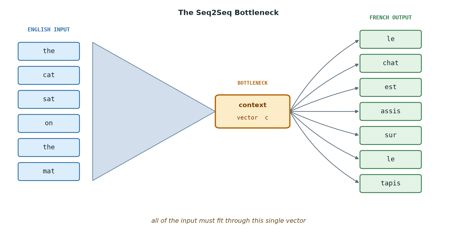
A left-to-right diagram showing an English input sentence flowing through a funnel into a single small box labelled "context vector", which then expands out to a French output sentence on the right. Arrows show each output word emerging one at a time from the context. A small note below the funnel reads "all of the input must fit through this single vector".

The whole input has to fit through that narrow point in the middle. For a 5-word sentence it works fine. For a 50-word sentence, things start falling out. That bottleneck is the central problem of seq2seq - and the reason attention was invented.

How it works

Encoder

The encoder is an RNN (or LSTM, or GRU) that reads the input sequence one token at a time and produces a hidden state at every step, exactly like the RNNs from the previous post. At the end of the input, the encoder’s final hidden state is taken as a summary of the whole input. That final state is called the context vector and gets handed off to the decoder.

context = encoder(input_sequence)   # final hidden state of the encoder

If you’ve ever written JSON.stringify(obj) to send something over a network, the encoder is the same idea - turn a structured input into a compact representation. The difference is that this one is lossy: the encoder doesn’t promise the input can be perfectly reconstructed, only that a useful summary of it is captured.

Decoder

The decoder is a separate RNN that generates the output sequence one token at a time, starting from the context vector. At each step it takes:

The previous decoder hidden state (initialised from the context vector)
The previously generated output token

…and produces:

A new hidden state
A distribution over the vocabulary for the next token

To pick the actual next token, the decoder takes the argmax of that distribution (greedy decoding) or samples from it. Generation begins with a special start token, written as <sos> (“start of sequence”), and continues until the decoder emits a special end token <eos> (“end of sequence”). The decoder learns when to stop by producing <eos> - there’s no other stopping rule.

The CS analogy: this is JSON.parse running on the compressed representation the encoder produced. Except it streams the output rather than returning it all at once.

Teacher forcing

During training, there’s a small trick that makes the decoder learn faster. At every step, the decoder needs to know the previous output token. If you feed it its own previous prediction, then a single wrong token early on cascades into garbage for the rest of the sequence - gradients become noisy and training is slow.

The fix is teacher forcing: during training, feed the decoder the correct previous token from the ground-truth output, regardless of what it actually predicted. The decoder always sees a clean history, the loss signal is sharp, and training converges much faster.

At inference time you don’t have the ground truth, so the decoder is forced to feed itself - predict a token, feed it back, predict the next, repeat. This is one reason small early errors are especially damaging at inference: there’s no teacher to correct them.

The bottleneck

Look at the encoder again. Whatever the input length - 5 tokens or 500 - the only thing that crosses over to the decoder is the final hidden state. That’s a single fixed-size vector. If the hidden size is 512, then 512 floats is all the information the decoder gets about the entire input.

512 floats is enough capacity for a short sentence. It is not enough for a paragraph. The encoder is forced to compress everything into a fixed budget regardless of input length, which means early tokens get overwritten as the encoder reads more, and late tokens dominate the final state. Translating a 50-word sentence, the first few words are often lost by the time generation begins.

This is the same issue you’d hit if you serialised an arbitrarily large object into a fixed-length buffer. Small objects fit. Big ones get truncated or overwritten. The math doesn’t care that you wanted to keep the early bytes - it runs out of room.

You can see this empirically: BLEU scores (the standard translation quality metric) for early seq2seq models fell off a cliff once sentences got longer than ~20 words. The architecture itself was the bottleneck.

The fix that became Section 2

The diagnosis: forcing one fixed vector to hold the entire input is the problem. The fix is to not do that. Instead of only passing the final encoder state to the decoder, pass all encoder hidden states - one per input token - and let the decoder decide at each generation step which encoder states it wants to look at.

That mechanism is called attention. The decoder, at each step, computes a weighted average over all encoder hidden states. The weights are learned and change per step: when generating “chat” in “le chat est assis”, the decoder pays most attention to the encoder state corresponding to “cat”. When generating “assis”, it shifts attention to “sat”. The fixed context bottleneck disappears because there’s no fixed context anymore - the decoder reads the whole input dynamically at every step.

Attention added to seq2seq broke the long-sentence wall and became the dominant NLP architecture from ~2015 to ~2017. Then someone asked the obvious question: if attention is so useful, why bother with the recurrent backbone at all? Drop the RNNs entirely, do everything with attention. That model is called the Transformer - and that’s where Section 2 begins.

Code

Step 1 - encoder forward pass:

A tiny LSTM encoder. We’ll feed it a 5-token English sentence and look at the final hidden + cell state - the context that gets handed to the decoder.

import torch
import torch.nn as nn

torch.manual_seed(0)

vocab_size, embed_dim, hidden = 20, 8, 16

class Encoder(nn.Module):
    def __init__(self):
        super().__init__()
        self.embed = nn.Embedding(vocab_size, embed_dim)
        self.lstm  = nn.LSTM(embed_dim, hidden, batch_first=True)

    def forward(self, input_ids):
        x = self.embed(input_ids)             # (batch, seq, embed)
        outputs, (h, c) = self.lstm(x)
        # outputs: (batch, seq, hidden) - one hidden state per input token
        # h, c:    (1, batch, hidden) - final hidden + cell state - the context
        return outputs, (h, c)

encoder = Encoder()
english = torch.tensor([[3, 7, 1, 12, 4]])    # 5-token "sentence", batch of 1
enc_outputs, context = encoder(english)

print(f"per-step encoder outputs: {enc_outputs.shape}")
print(f"context hidden:           {context[0].shape}")
print(f"context cell:             {context[1].shape}")

per-step encoder outputs: torch.Size([1, 5, 16])
context hidden:           torch.Size([1, 1, 16])
context cell:             torch.Size([1, 1, 16])

The per-step outputs are 5 × 16 (one 16-dim vector per token). The context is a single 16-dim vector - the encoder’s final state. That single vector is all the decoder will see of the input.

Step 2 - decoder forward pass:

The decoder is another LSTM, initialised from the encoder’s context, generating one token at a time.

class Decoder(nn.Module):
    def __init__(self):
        super().__init__()
        self.embed = nn.Embedding(vocab_size, embed_dim)
        self.lstm  = nn.LSTM(embed_dim, hidden, batch_first=True)
        self.out   = nn.Linear(hidden, vocab_size)

    def forward(self, prev_token, state):
        x = self.embed(prev_token)             # (batch, 1, embed)
        out, state = self.lstm(x, state)
        logits = self.out(out.squeeze(1))      # (batch, vocab)
        return logits, state

decoder = Decoder()
SOS, EOS, MAX_LEN = 0, 1, 8

# start decoding from the encoder's final state
state = context
prev  = torch.tensor([[SOS]])
generated = []

for step in range(MAX_LEN):
    logits, state = decoder(prev, state)
    next_token = logits.argmax(dim=-1)         # greedy decode
    if next_token.item() == EOS:
        break
    generated.append(next_token.item())
    prev = next_token.unsqueeze(0)

print(f"generated token ids: {generated}")

generated token ids: [10, 10, 10, 10, 10, 10, 10, 10]

The model is untrained, so the output is gibberish - the same token over and over. But the mechanics are what matter: a token in, a token out, looping until <eos> (or a length cap). This is how every autoregressive language model - including modern LLMs - generates text.

Step 3 - the bottleneck, visualised:

The context vector has the same size no matter how long the input is. We can verify this directly.

for length in [3, 10, 50, 200]:
    input_ids = torch.randint(0, vocab_size, (1, length))
    _, (h, c) = encoder(input_ids)
    print(f"input length {length:>3}  →  context shape: {tuple(h.shape)}")

input length   3  →  context shape: (1, 1, 16)
input length  10  →  context shape: (1, 1, 16)
input length  50  →  context shape: (1, 1, 16)
input length 200  →  context shape: (1, 1, 16)

Three tokens or two hundred - the encoder hands the decoder exactly 16 numbers. The math doesn’t grow the context to match the input. That mismatch - fixed-size container, variable-size content - is the bottleneck Section 2 fixes.

Key takeaways

Seq2Seq glues two RNNs together - an encoder that compresses the input into a single context vector, and a decoder that generates a new sequence from it. This let one model handle variable input and variable output lengths.
During training, the decoder uses teacher forcing - it’s fed the ground-truth previous token instead of its own prediction so the loss signal stays clean. At inference the decoder feeds itself, which makes early errors especially damaging.
The fixed-size context vector is a hard bottleneck: long inputs get squashed and information from early tokens gets lost. Attention removes this bottleneck by letting the decoder look at all encoder states dynamically - and is the foundation of the Transformer.

What to read next

We’ve reached the end of Section 1. You now have the full mental model of pre-Transformer deep learning: feedforward networks, optimisers, regularisation, the architectures shaped to their inputs, and the bottleneck that forced the next generation of models to do something new.

Section 2 starts there. The next post is about attention - the mechanism that fixed seq2seq’s bottleneck, and the single idea that the entire Transformer is built around.

→ Post 2.1 - The Attention Mechanism