Posts 1.1–1.8 gave us the building blocks: neurons, activations, losses, gradients, optimisers, normalisation, regularisation. That’s enough to train a feedforward network on tabular data. But most interesting data isn’t tabular - it’s images, audio, text, time series. This post walks through the three architectures that came before Transformers and the specific problem each one tried to solve.
Why it exists
A standard feedforward network expects a fixed-size input. Twenty features in, ten features out. That’s fine for predicting house prices from 20 columns of a spreadsheet. But:
- An image is a 2D grid of pixels. Treating each pixel as an independent feature throws away the fact that nearby pixels are related - an edge in a face spans several adjacent pixels.
- A sentence is a sequence of words of variable length. “Hi” and “The quick brown fox jumped over the lazy dog” are both valid inputs, but they have wildly different sizes.
- Audio is a long time series - tens of thousands of samples per second.
A feedforward network has no built-in idea of “next to” or “in sequence with”. You have to bake that structure into the architecture. Three big attempts came before Transformers - each one fixing a real problem in the previous, each one creating a new one.
CNNs (Convolutional Neural Networks) handled spatial structure for images. RNNs (Recurrent Neural Networks) handled sequences for text and audio. LSTMs (Long Short-Term Memory networks) fixed a numerical problem in RNNs. None of them won in the end - but understanding what each failed at is what makes the Transformer’s design choices make sense.
Intuition
The shape that matters most for this post is the RNN. Unroll it across time and you see how a single recurrent cell processes a sequence: the same weights, applied step after step, with a hidden state passed forward.
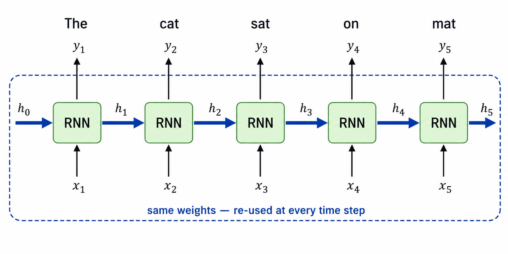
The picture tells you the whole story. There is one cell. It runs N times for a sequence of length N. At each step it sees a new input and the previous hidden state, and produces a new hidden state. The hidden state is the only memory the network has of what came before.
That single arrow flowing left to right is also where the trouble starts - but we’ll get to that.
How it works
CNN - for spatial data
A CNN scans an image with a small filter (also called a kernel) - typically a 3×3 or 5×5 patch of learnable weights. The filter slides across the image, computing a dot product at every position. The result is a new image (called a feature map) where each pixel summarises a small neighbourhood of the original.
If you’ve ever written a sliding-window algorithm - sliding-window max, a moving average over an array - that’s the operation. The CNN learns what to compute in each window, instead of you specifying it.
A single 3×3 filter has 9 learnable weights plus one bias - 10 numbers total. A real CNN layer learns many filters in parallel (often 32, 64, or 128), each looking for a different pattern. One filter might fire on vertical edges, another on horizontal ones, another on a blob of red. The output of the layer is a stack of feature maps, one per filter.
There are three knobs that control how the filter slides:
- Stride - how many pixels to jump between positions. Stride 1 produces one output per input pixel (a feature map roughly the same size as the input). Stride 2 jumps every other pixel - the output is half as wide and half as tall. Higher stride = aggressive downsampling.
- Padding - what to do at the edges. A 3×3 filter centred on a corner pixel falls off the edge of the image, so without help it can’t be applied there. The fix is to add a ring of zeros around the input so the filter has room. With
padding=1and a 3×3 kernel, a 28×28 input produces a 28×28 output (same size). Without padding, every layer shaves pixels off each side and your image shrinks one row and one column at a time. - Channels - colour images have 3 input channels (R, G, B). A 3×3 filter on a 3-channel input actually has 3×3×3 = 27 weights - one 3×3 patch per channel - and the dot product sums across all of them to produce one output value. Stacked layers grow channel count further: a layer with 64 filters produces a 64-channel output, and the next layer’s filters span across all 64.
After a few convolutional layers, a CNN typically uses pooling to shrink the spatial size. The most common is max pooling: take a 2×2 window, output the maximum value in it, slide on. A 28×28 feature map becomes 14×14. Pooling makes the model less sensitive to exact pixel positions (a small shift in the input doesn’t change which value is the max) and roughly quarters the work the next layer has to do.
The patch in the original image that each output pixel ultimately “sees” is called its receptive field. A single 3×3 filter sees a 3×3 patch. Stack two 3×3 conv layers and each output sees a 5×5 patch. Stack ten and you cover most of an image. Pooling accelerates this - every 2×2 pool doubles the receptive field for free.
A typical small CNN looks like Conv(3→32) → Pool → Conv(32→64) → Pool → Conv(64→128) → Pool → Flatten → Linear → softmax. By the time the input reaches the linear layer, it has gone from a 28×28×1 raw image down to perhaps 3×3×128 - a compact summary of the patterns the convolutions found.
Why this works for images: a cat is still a cat whether it appears in the top-left or bottom-right of the photo. A CNN’s filters look the same everywhere, so the model is translation invariant. Stack a few CNN layers and you get a hierarchy: early layers detect edges, middle layers detect textures, late layers detect whole shapes.
CNNs took over computer vision in the 2010s. They’re still the right tool when your input has 2D structure and locality matters. But they don’t naturally handle sequences - a 3×3 filter has no concept of “the third word vs the first word” because text isn’t a grid, it’s an ordered list. You can apply 1D convolutions to text and it works for short-range patterns, but the locality assumption (nearby tokens are what matter most) breaks down for sentences where the subject and verb can be 20 words apart.
RNN - for sequences
An RNN processes a sequence one element at a time. At each step t, it takes the current input x_t and the previous hidden state h_{t-1}, and produces the new hidden state h_t:
h_t = tanh(W_x · x_t + W_h · h_{t-1} + b)Let’s pin down the shapes so the equation isn’t only symbols. Say each input is a 4-dimensional vector (a one-hot for a 4-word vocabulary, or a 4-dim embedding) and the hidden state has 6 dimensions. Then W_x is a 6×4 matrix (maps input to hidden), W_h is a 6×6 matrix (maps hidden to hidden), and b is a 6-vector. The output h_t is 6-dimensional. Those three tensors - W_x, W_h, b - are the only learnable parameters in the cell, and they are reused at every step.
Why tanh? Because the cell mixes two signals - the current input and the previous hidden state - and the result needs to stay bounded. tanh squashes everything into [-1, 1]. Without it, multiplying by W_h over and over would let the hidden state grow without limit and the network would blow up.
The initial hidden state h_0 is a vector of zeros by convention - no memory before the sequence starts. You start fresh at the first step.
The hidden state acts as a running summary of everything the network has seen so far. The mental model from your CS coursework: this is a reduce over a stream. array.reduce((state, item) => update(state, item), initial). The hidden state is the accumulator, the RNN cell is the reducer function, the sequence is the stream.
How you use the RNN depends on the shape of the task:
- Many-to-one: take only the final hidden state and feed it into a classifier. Used for sentiment analysis - read the whole sentence, emit one label at the end.
- Many-to-many (aligned): feed each step’s hidden state into an output head. Used for part-of-speech tagging - one input token, one output prediction, parallel structure.
- Many-to-many (unaligned): input and output sequences have different lengths, like translation (“Hello, world” → “Bonjour, monde”). This needs the encoder-decoder setup we’ll cover in the next post.
Two common extensions: you can stack RNN layers - feed the hidden states of one RNN as inputs to another. Common in practice and what nn.RNN(..., num_layers=2) does. And you can run a second RNN backward over the same sequence to get a bidirectional RNN, where each token’s representation sees both past and future context. Bidirectional works well for tagging tasks but not for generation - you can’t see the future when generating one token at a time.
That gives RNNs a few nice properties. They handle variable-length input - run more steps. They can in principle remember arbitrary history - the hidden state is supposed to summarise everything. And they parameter-share across positions - the same cell handles word 1 and word 100.
In principle. In practice they run into a wall called the vanishing gradient problem.
Vanishing gradient - why RNNs forget
To train an RNN you do backpropagation through time (often shortened to BPTT) - unroll the network across all T steps and backprop the gradient from the final output back through every step. The chain rule kicks in at every step, multiplying gradients together.
Concretely, the gradient of the loss with respect to the hidden state at step t is a product of jacobians, one for each step from T back down to t:
∂L/∂h_t = ∂L/∂h_T · ∂h_T/∂h_{T-1} · ∂h_{T-1}/∂h_{T-2} · ... · ∂h_{t+1}/∂h_tThat’s T - t matrix multiplications stacked back to back. Each per-step jacobian ∂h_{k+1}/∂h_k works out to W_h^T element-wise multiplied by tanh'(z_k) - the derivative of tanh, which is a number between 0 and 1 (and approaches 0 whenever the neuron is saturated, i.e. when its pre-activation z_k is large in either direction).
So the magnitude of the gradient at step t is roughly the magnitude of (W_h^T · diag(tanh'))^(T-t). Two things govern how that behaves:
- The largest eigenvalue of
W_h- called its spectral radius. If it’s less than 1, repeated multiplication contracts everything toward zero. If it’s greater than 1, it blows up. Right at 1, gradients stay roughly the same size - but that’s a knife-edge condition and impossible to tune to in practice. tanh'(z)is at most 1, and is much smaller whenever the neuron is saturated. So even with a perfectly tunedW_h, the activation derivative drags the per-step factor below 1.
If the combined per-step factor has magnitude ~0.5, then over 20 steps you’ve multiplied 0.5 by itself 20 times. That’s roughly 1e-6. The gradient that should be updating the weights for step 1 is now numerically indistinguishable from zero - the optimiser sees no signal to update on, and the network can’t learn anything about long-range context.
This is exactly the same kind of underflow that bites you when multiplying many small floating-point numbers. The math is fine in theory. The numbers collapse.
The mirror-image problem is exploding gradients - if each step’s local factor is 1.5, then 1.5^20 ≈ 3000, and one update sends your weights to nonsense values. Exploding gradients can be patched with gradient clipping - cap the gradient’s magnitude before the optimiser step - because rescaling brings the gradient back into a safe range without changing its direction. Vanishing gradients are harder to fix from outside: rescaling a 1e-9 gradient up doesn’t help, because the direction it points in has already lost information from being squashed through many multiplications. You have to redesign the cell so the gradient never gets squashed in the first place.
People tried partial fixes - using ReLU instead of tanh (its derivative is exactly 1 in the positive region), more careful weight initialisation, gradient clipping - but none of them fully solved the problem for sequences longer than a few dozen steps. The real fix was to give the gradient a different path through the cell entirely. That fix is the LSTM.
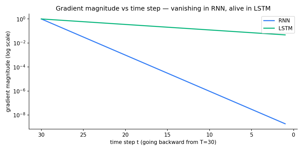
The plot above shows the gradient magnitude at every step of a 30-step sequence, going from the final loss backward. The RNN curve drops by 12 orders of magnitude. The LSTM curve stays roughly flat. That difference is the whole reason LSTMs replaced plain RNNs.
LSTM - gates that keep gradients alive
The LSTM keeps the same skeleton - process one step at a time, carry state forward - but adds two things:
- A separate cell state
c_tthat flows through the network with very little modification. This is the “highway” that gradients can travel along without being squashed. - Three gates that decide what to do to that cell state at each step.
Each gate is a tiny one-layer network. It takes the previous hidden state and current input, runs them through a linear layer, and applies the sigmoid function - written σ - which maps any real number into [0, 1]. The output is a vector of numbers in that range. Element-wise: a gate value of 0 for a given dimension means “block this dimension”, a value of 1 means “let it pass”. Every dimension of the state has its own gate value, so the LSTM can keep some features and forget others independently in the same step.
The full equations for one LSTM step:
f_t = σ(W_f · [h_{t-1}, x_t] + b_f)     # forget gate
i_t = σ(W_i · [h_{t-1}, x_t] + b_i)     # input gate
g_t = tanh(W_g · [h_{t-1}, x_t] + b_g)  # candidate values
o_t = σ(W_o · [h_{t-1}, x_t] + b_o)     # output gate

c_t = f_t * c_{t-1} + i_t * g_t          # update cell state
h_t = o_t * tanh(c_t)                    # new hidden state
[h_{t-1}, x_t] means “concatenate the previous hidden state with the current input into one long vector”. The four W matrices and four b vectors are the learnable parameters. Compared to a plain RNN - which has only W_x, W_h, b - an LSTM has roughly 4× as many parameters per cell, because each gate gets its own copy.
Walking through one step:
- Forget gate
f_tlooks at the previous hidden state and current input, then outputs a value in[0, 1]for each dimension of the cell state. That value is the fraction of the old cell state to keep.f_t[i] = 0.9means “keep 90% of dimension i”.f_t[i] = 0wipes that dimension. - Input gate
i_tdecides how much of the new candidateg_tto write into the cell state.g_titself is a fresh suggestion for what the cell state could contain at this step, computed from the current input and the previous hidden state (and squashed by tanh so its values stay in[-1, 1]). - Cell update
c_t = f_t * c_{t-1} + i_t * g_tis the heart of the LSTM. It’s an additive update - old state scaled down, plus new information scaled up. There is no matrix multiplication betweenc_{t-1}andc_t, only element-wise multiplies. - Output gate
o_tdecides what part of the updated cell state to expose ash_t- which is what gets passed to the next step and into any output layer above.
Two things to notice about the cell-state update. First, c_t is a direct function of c_{t-1}, scaled by the forget gate - there’s no W_h matrix between them. Second, when the forget gate is open (close to 1), the gradient flows back through c_{t-1} almost untouched. Gradients can travel back tens or hundreds of steps before they vanish.
The CS analogy is a controlled write to shared memory. The forget gate is “should I keep the old value?”, the input gate is “should I write a new value?”, and the cell state is the memory cell itself. Plain RNNs were forced to rewrite the whole state every step. LSTMs can choose to leave it alone.
A simplified cousin called the GRU (Gated Recurrent Unit) merges some of these gates - it has only two (a reset gate and an update gate) and no separate cell state. Fewer parameters, often comparable quality, popular as a lighter alternative when LSTMs are overkill.
What still wasn’t right
LSTMs trained well. They drove the state of the art in machine translation, speech recognition, and language modelling for several years. But two problems remained:
- No parallelism. To compute the hidden state at step 100, you have to first compute steps 1 through 99, in order. You cannot use the GPU’s ability to process many things at once - every step depends on the previous one. Training on long sequences is painfully slow.
- Still a fixed memory. Even with gates, the cell state is a fixed-size vector. Cramming an entire book’s context into 512 numbers is hard. The model has to choose what to forget, and it sometimes chooses wrong.
The first problem is the one that hurt at scale. Imagine a for loop that can’t be parallelised - you’re stuck with single-threaded performance no matter how big your GPU is. Transformers fix this directly: they replace the sequential for loop with a single big parallel operation called attention, which we’ll get to in section 2.
Code
Step 1 - RNN forward pass, one step at a time:
We’ll process the 5-word sentence “the cat sat on mat” through a tiny RNN by hand. Each word becomes a 4-dim vector (one-hot for now). The hidden state has size 6.
import numpy as np

np.random.seed(0)
vocab = ["the", "cat", "sat", "on", "mat"]
H = 6  # hidden size
W_x = np.random.randn(H, len(vocab)) * 0.1
W_h = np.random.randn(H, H) * 0.1
b   = np.zeros(H)

def rnn_step(x_t, h_prev):
    return np.tanh(W_x @ x_t + W_h @ h_prev + b)

h = np.zeros(H)
for word in vocab:
    x = np.eye(len(vocab))[vocab.index(word)]  # one-hot
    h = rnn_step(x, h)
    print(f"after '{word}':  h = {np.round(h, 3)}")
after 'the': h = [-0.058 -0.018 0.034 0.155 0.085 -0.039]
after 'cat': h = [ 0.026 -0.072 0.124 0.236 0.064 0.04 ]
after 'sat': h = [-0.061 0.171 0.085 0.181 0.182 -0.012]
after 'on': h = [-0.046 0.114 0.149 0.265 0.105 -0.071]
after 'mat': h = [ 0.025 -0.005 0.166 0.252 0.072 0.072]The hidden state changes at every step, but the weights are identical at every step. Whatever the network has learned is baked into W_x, W_h, b once - it gets reused for every position in the sequence.
Step 2 - vanishing gradient on a long sequence:
Each backward step through an RNN multiplies the gradient by the recurrent weight matrix W_h^T and by tanh'. For a stably-initialised RNN, the combined per-step factor is less than 1 - call it about 0.5. After 30 steps, the gradient has shrunk by 0.5^30 ≈ 1e-9.
An LSTM’s cell-state path looks different. The gradient is carried mainly through the forget gate, which is typically open (~0.9), and there is no big matrix multiplication in between to shrink it. The per-step factor stays close to 1.
import numpy as np
import matplotlib.pyplot as plt

T = 30
rnn_per_step  = 0.5   # ‖W_h^T‖ · ‖tanh'‖ for a typical stably-initialised RNN
lstm_per_step = 0.9   # forget gate ≈ 0.9, no big matrix multiplication

rnn_norms  = [rnn_per_step  ** i for i in range(T)]
lstm_norms = [lstm_per_step ** i for i in range(T)]

steps = np.arange(T, 0, -1)
plt.figure(figsize=(8, 4))
plt.semilogy(steps, rnn_norms,  label="RNN",  color="#3b82f6", lw=2)
plt.semilogy(steps, lstm_norms, label="LSTM", color="#10b981", lw=2)
plt.xlabel("time step t (going backward from T=30)")
plt.ylabel("gradient magnitude (log scale)")
plt.title("Gradient magnitude vs time step - vanishing in RNN, alive in LSTM")
plt.legend()
plt.gca().invert_xaxis()
plt.tight_layout()
plt.savefig("assets/images/1.9/vanishing-gradient.png", dpi=150)
plt.show()
RNN gradient at earliest step: 1.86e-09
LSTM gradient at earliest step: 0.047The RNN gradient at step 1 is essentially numerical zero - the optimiser has no signal to update on. The LSTM still has 5% of the original magnitude after 30 steps, which is plenty for training. This is the whole reason gates exist - they give gradients a path that doesn’t get squashed.
Step 3 - nn.RNN and nn.LSTM in PyTorch:
In practice you don’t roll the loop yourself. PyTorch ships both:
import torch
import torch.nn as nn

batch, seq_len, input_size, hidden_size = 2, 5, 4, 6

x = torch.randn(batch, seq_len, input_size)

rnn  = nn.RNN(input_size,  hidden_size, batch_first=True)
lstm = nn.LSTM(input_size, hidden_size, batch_first=True)

rnn_out,  rnn_h        = rnn(x)
lstm_out, (lstm_h, lstm_c) = lstm(x)

print(f"RNN output shape:  {rnn_out.shape}    final hidden: {rnn_h.shape}")
print(f"LSTM output shape: {lstm_out.shape}    final hidden: {lstm_h.shape}    cell: {lstm_c.shape}")
RNN output shape: torch.Size([2, 5, 6]) final hidden: torch.Size([1, 2, 6])
LSTM output shape: torch.Size([2, 5, 6]) final hidden: torch.Size([1, 2, 6]) cell: torch.Size([1, 2, 6])The shapes tell the story. The output has one vector per time step (length 5). The RNN also returns one final hidden state. The LSTM returns a final hidden state and a final cell state - that extra cell state is the gradient highway.
Key takeaways
- CNNs handle spatial locality with sliding filters; RNNs handle sequences with a hidden state that carries memory forward. Each is shaped by the structure of its input.
- Plain RNNs suffer from vanishing gradients - multiply many small numbers and the signal for early steps disappears. LSTMs fix this with a cell state and three gates that let gradients flow across long distances.
- LSTMs still process one step at a time, so they cannot exploit GPU parallelism. This is the bottleneck Transformers were designed to remove.
What to read next
LSTMs got us as far as a single sequence in, single sequence out. But many real tasks - translation, summarisation, question answering - are sequence-to-sequence with different input and output lengths. The next post covers the seq2seq architecture, the fixed-size bottleneck it created, and the one idea that finally fixed it.
→ Post 1.10 - Seq2Seq: Teaching Machines to Translate