In post 1.5 we set up a good optimizer - AdamW with adaptive learning rates and weight decay. But there’s a separate problem that shows up as networks get deeper: the values flowing through the network drift over time. This post is about why that happens and how normalisation fixes it.
Why it exists
Run a 20-layer network with no normalisation and look at the distribution of values coming out of each layer. Layer 1 might output values between -1 and 1. By layer 10, the values are in the thousands. By layer 20, they’ve either exploded to huge numbers or collapsed to near-zero.
This happens because each layer multiplies its inputs by its weights. If a layer’s weights are slightly greater than 1, the values grow with every pass. Slightly less than 1, they shrink. Over 20 layers, small multiplicative errors compound - the same reason 1.01^20 ≈ 1.22 and 0.99^20 ≈ 0.82.
Exploding or vanishing values cause two problems. First, gradient descent breaks: gradients computed on huge or tiny activations are unstable, and training either diverges or stalls. Second, activations saturate: if your activation function (like sigmoid) is given a value of 1000, it outputs 1.0 for everything, and you’ve lost all information about the input.
Normalisation fixes this by rescaling the activations at each layer so they have a predictable distribution - roughly zero mean and unit variance - before passing to the next layer.
The formula is z-score standardisation, the same thing you’ve seen in statistics or data preprocessing:
x_normalised = (x - mean) / sqrt(variance + ε)ε is a small number added to prevent dividing by zero.
After normalising, a learned scale (γ) and shift (β) are applied to give the network the freedom to undo the normalisation if needed:
output = γ × x_normalised + βγ and β are learnable parameters, just like weights. This means the network can learn “actually, this layer works better with a mean of 2 and a variance of 3” - the normalisation step doesn’t force a rigid distribution, it just stabilises the starting point.
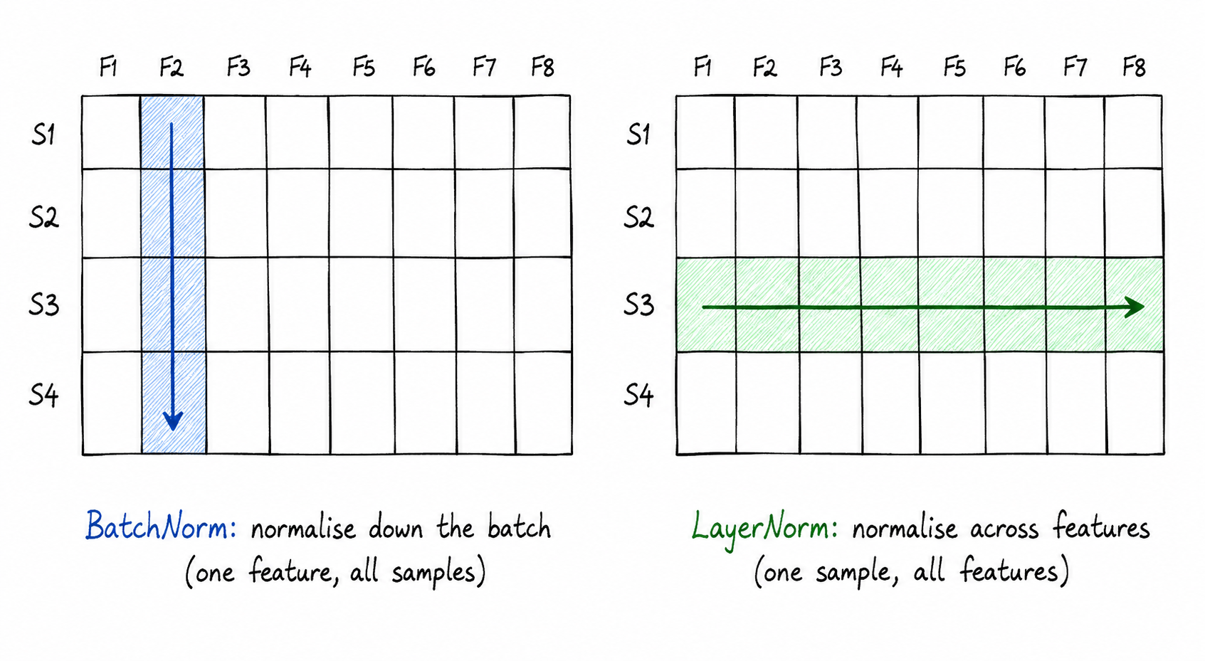
The question is: what values do you compute mean and variance over? That’s what separates BatchNorm from LayerNorm.
How it works
BatchNorm
BatchNorm (Batch Normalisation) computes mean and variance across the batch dimension.
Say your batch has 64 samples, and each sample has 512 features. BatchNorm looks at each of the 512 features and asks: across all 64 samples in this batch, what’s the mean and variance of this feature? Then it normalises using those batch-level statistics.
The key word is “across the batch.” BatchNorm’s normalisation stats depend on the other samples sharing the batch with you.
That’s fine for image models. Images are all the same size, batch sizes are large enough to compute stable statistics, and inference can use running averages collected during training.
But it breaks in two situations:
- Batch size of 1. If you have one sample, the mean and variance are that one sample’s values - you haven’t actually normalised anything meaningful.
- Variable-length sequences. A sentence of 5 words and a sentence of 500 words can’t share meaningful statistics across a batch. The activations represent fundamentally different positions in a sequence.
Think of it like a global lock in concurrent programming. BatchNorm requires all samples in the batch to coordinate to compute a shared statistic before any single sample can proceed. That works when all inputs are the same shape - but it’s a bottleneck when inputs differ, and it fails entirely when you have nothing to aggregate across.
LayerNorm
LayerNorm (Layer Normalisation) computes mean and variance across the feature dimension of a single sample.
For one sample with 512 features, LayerNorm looks at all 512 values and normalises them using their own mean and variance - no other samples involved.
Every sample normalises itself. Batch size doesn’t matter. Sequence length doesn’t matter. Whether you’re at training time or inference time, the statistics are computed from the sample you’re currently processing.
That’s why transformers use LayerNorm. Text sequences vary in length. Batching sequences together requires padding shorter ones to match the longest, which already complicates batch statistics. LayerNorm sidesteps all of this - each token normalises its own 512-dimensional vector without consulting anything else.
There’s no global state. No coordination across samples. Like a function that only reads its own local variables - nothing shared, nothing to synchronise.
RMSNorm
RMSNorm (Root Mean Square Normalisation) is a simplified version of LayerNorm used in LLaMA, Mistral, and most modern open-source LLMs.
Standard LayerNorm subtracts the mean before scaling (centring + scaling). RMSNorm skips the centring and just scales by the root mean square:
RMS(x) = sqrt(mean(x²))
x_normalised = x / RMS(x)
No mean subtraction - just divide by the magnitude. The intuition: centering is often redundant because the scale parameter (γ) can implicitly shift the distribution. Removing it shaves compute without hurting quality.
If LayerNorm is “normalise by subtracting mean and dividing by standard deviation,” RMSNorm is “just divide by the typical magnitude.” One fewer thing to compute, similar results in practice.
Code
Step 1 - watch activations drift without normalisation:
A 10-layer network, each layer a Linear + ReLU. No normalisation. We’ll plot the distribution of activations at layer 1, layer 5, and layer 10.
import torch
import torch.nn as nn
import matplotlib.pyplot as plt

torch.manual_seed(42)

class DeepNetNoNorm(nn.Module):
    def __init__(self, depth=10, width=256):
        super().__init__()
        self.layers = nn.ModuleList([
            nn.Sequential(nn.Linear(width, width), nn.ReLU())
            for _ in range(depth)
        ])

    def forward(self, x):
        snapshots = {}
        for i, layer in enumerate(self.layers):
            x = layer(x)
            if i in (0, 4, 9):
                snapshots[f"layer {i+1}"] = x.detach().flatten().numpy()
        return x, snapshots

model = DeepNetNoNorm()
x = torch.randn(64, 256)  # batch of 64 samples, 256 features
_, snapshots = model(x)

fig, axes = plt.subplots(1, 3, figsize=(12, 3))
for ax, (name, values) in zip(axes, snapshots.items()):
    ax.hist(values, bins=60, color="#3b82f6", alpha=0.8)
    ax.set_title(f"{name}  (std={values.std():.1f})")
    ax.set_xlabel("activation value")
    ax.spines["top"].set_visible(False)
    ax.spines["right"].set_visible(False)

plt.suptitle("Activations without normalisation — distribution shifts across layers")
plt.tight_layout()
plt.savefig("/images/posts/batchnorm-vs-layernorm/activations-no-norm.png", dpi=150)
plt.show()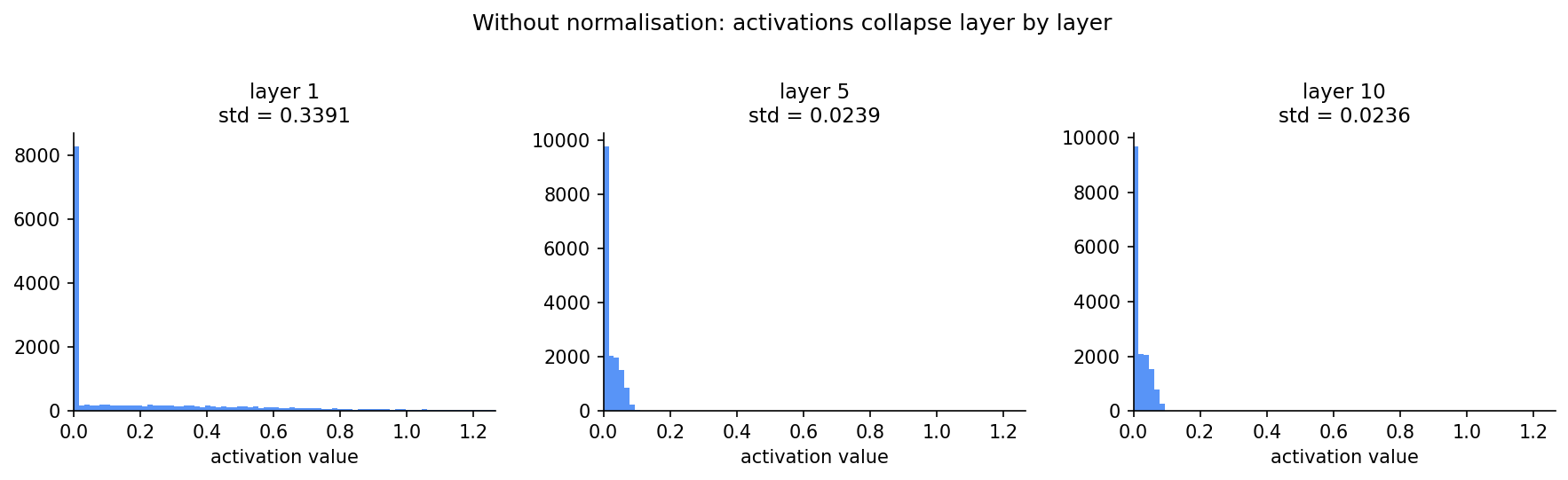
With the same x-axis across all three, the collapse is clear. Layer 1 has a spread of values reaching up to 1.2. By layer 5, almost everything is crushed into a spike near zero and stays there. The standard deviation drops from 0.34 to 0.02 in five layers.
Step 2 - add LayerNorm and watch the distributions stabilise:
class DeepNetWithLayerNorm(nn.Module):
    def __init__(self, depth=10, width=256):
        super().__init__()
        self.layers = nn.ModuleList([
            nn.Sequential(nn.Linear(width, width), nn.LayerNorm(width), nn.ReLU())
            for _ in range(depth)
        ])

    def forward(self, x):
        snapshots = {}
        for i, layer in enumerate(self.layers):
            x = layer(x)
            if i in (0, 4, 9):
                snapshots[f"layer {i+1}"] = x.detach().flatten().numpy()
        return x, snapshots

model_norm = DeepNetWithLayerNorm()
torch.manual_seed(42)
x = torch.randn(64, 256)
_, snapshots_norm = model_norm(x)

fig, axes = plt.subplots(1, 3, figsize=(12, 3))
for ax, (name, values) in zip(axes, snapshots_norm.items()):
    ax.hist(values, bins=60, color="#10b981", alpha=0.8)
    ax.set_title(f"{name}  (std={values.std():.1f})")
    ax.set_xlabel("activation value")
    ax.spines["top"].set_visible(False)
    ax.spines["right"].set_visible(False)

plt.suptitle("Activations with LayerNorm — distribution stays consistent")
plt.tight_layout()
plt.savefig("/images/posts/batchnorm-vs-layernorm/activations-with-layernorm.png", dpi=150)
plt.show()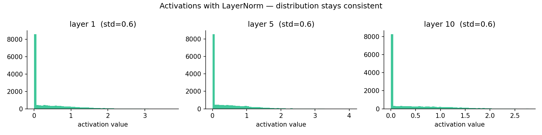
The distributions now look nearly identical across layers 1, 5, and 10. Gradients flowing back through a normalised network are much more stable.
Step 3 - using nn.LayerNorm in practice:
import torch
import torch.nn as nn

# normalise a batch of sequences: (batch=4, seq_len=10, features=64)
x = torch.randn(4, 10, 64)
norm = nn.LayerNorm(64)   # normalise the last dimension (features)

out = norm(x)
print(f"input  shape: {x.shape}")
print(f"output shape: {out.shape}")
print(f"input  mean={x.mean():.3f}  std={x.std():.3f}")
print(f"output mean={out.mean():.3f}  std={out.std():.3f}")
input shape: torch.Size([4, 10, 64])
output shape: torch.Size([4, 10, 64])
input mean=0.006 std=0.998
output mean=0.000 std=0.570Shape is unchanged - LayerNorm is applied in-place. The output mean is near zero and variance is tightened. You’d see a larger effect with deep, uninitialized networks where values have actually drifted.
nn.LayerNorm(64) tells PyTorch: “normalise the last 64 dimensions.” In a transformer this is called at every attention block and every feed-forward block. It’s one line, but it’s what keeps a 96-layer model trainable.
Key takeaways
- Activations drift as they flow through deep layers, making gradients unstable - normalisation rescales them at each layer to keep training stable
- BatchNorm normalises across the batch dimension (needs other samples), LayerNorm normalises across the feature dimension of a single sample (no batch dependency) - transformers use LayerNorm because text sequences vary in length
- RMSNorm is a simplified LayerNorm that skips mean subtraction - it’s what LLaMA and most modern open-source LLMs use
What to read next
Training is now stable thanks to normalisation. But there’s one more thing networks do to avoid overfitting: deliberately break during training so they don’t memorise the data.
→ Post 1.7 - Dropout and Overfitting